R Programming // Foundations May 5, 2022  

What Makes Some Algorithms Better and a First Look at Big O Notation

---

In our first code lab on Estimating Pi with Dart Throwing, we talked briefly about algorithms. If you’re new to algorithms, we can think of them as recipes, or instructions, for doing or computing something. Today, we’ll dive a little deeper into some aspects of algorithms.

Imagine that we did a quick search online and found a handful of recipes for baking the same cake. As you’d expect, not all of these recipes are equally good. Some may produce cakes with better texture or taste. Others might produce equally good cakes but require less work.

In the same way that some recipes are better than others, there are a number of things that can make some algorithms better than others. One of these things is how the amount of work required grows as we increase the size of the input data. Formally, this is called computational complexity.

How do we measure computational work or time?

We can make a very rough estimate of the amount of computational work or computational time a procedure requires by counting the number of basic arithmetic operations it involves. Also called floating point operations, these refer to the number of addition, subtraction, multiplication, and division operations that the algorithm requires.

Let’s look at a few simple examples so we can get a better sense of what this means.

Example 1: How much computational time does it take to compute the mean of \(n\) numbers?

Let’s say we want to compute the mean, or average, of \(n\) numbers. How much work does this involve? Let’s label each number as \(x_{1}, x_{2}, \dots\) and so on up to \(x_{n}\). Let’s call their average \(\bar{x}\). We read this as “x bar” and commonly compute it with the following formula

\[\bar{x} = \frac{1}{n}(x_{1} + x_{2} + \dots + x_{n}).\]

We can see that this requires \(n-1\) additions and \(1\) multiplication. So in total, there are \(n\) basic arithmetic operations, or flops. We write this as \(O(n)\) and read it as “Oh of \(n\)”.

This means that the above algorithm for computing the average scales linearly in the size of the data. By this, we mean that if we increase the value of \(n\) (so that we average more numbers), the number of basic arithmetic operations that the algorithm requires will grow by some factor of \(n\).

Let’s test this out in R!

Let’s take a look at this in R! If you’re new to R, I have a two-part series on getting started with coding in R (Part 1 and Part 2). That series will walk you through getting you up to speed in R so you can follow along with the code snippets here.

In the nlist object below, the values 1e5, 1e6, 1e7, 4e7, 6e7 and 1e8 are \(1\times 10^{5}, 1\times 10^{6}, 1\times 10^{7}, 4\times 10^{7}, 6 \times 10^{7}\), and \(1\times 10^{8}\), respectively. We’ll use the built-in R function mean() to take the average of \(n\) numbers.

We can use the system.time() function to time how long a procedure requires. The system.time() function outputs an object containing 3 values. These are the user time, system time, and total elapsed time in seconds. We’ll use the latter, or third element, to measure our time.

# Get varying values of n
nlist <- c(1e5, 1e6, 1e7, 4e7, 6e7, 1e8)

# Make output container
time <- numeric(length=length(nlist))

# Compute the mean for each value of n, record the time in seconds
for (a in 1:length(nlist)) {
  set.seed(123)
  numbers <- rnorm(nlist[a])
  time[a] <- system.time(mean(numbers))[3]
}

Let’s plot the timing results so we can see visually compare the increase in time with the increase in \(n\).

plot(nlist, time, xlab="n", ylab="Time in seconds",
     main="Time in seconds to compute the mean of n numbers",
     pch=16)
lines(nlist, time)

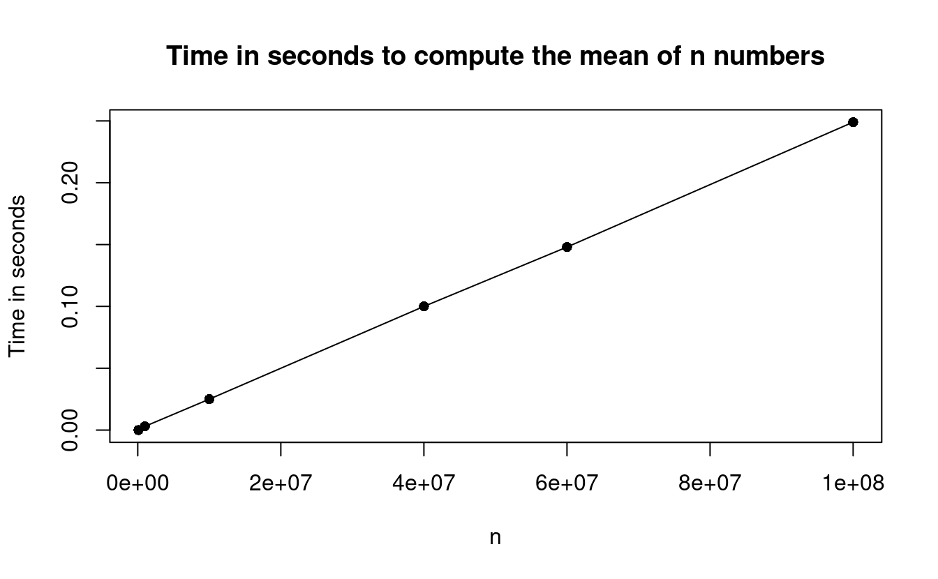
This plot illustrates how the mean() function is a linear time algorithm since it scales linearly in \(n\).

How much computational time does it take to compute the variance of \(n\) numbers?

Suppose we want to compute the variance of \(n\) numbers. Again, we’ll label the numbers \(x_{1}, x_{2}, \dots, x_{n}\). This time, let’s call the variance \(v\). We can compute this with the following formula

\[v = \frac{1}{n-1}\sum_{i=1}^{n} (x_{i} - \bar{x})^{2}.\]

If you’re unfamiliar with the summation notation above, it means that we will sum \((x_{i}-\bar{x})^{2}\) for all integers \(i\) that range from \(1\) to \(n\) (including those end numbers). This is a more compact way of writing the following

\[\sum_{i=1}^{n} (x_{i} - \bar{x})^{2} = (x_{1}-\bar{x})^{2} + (x_{2}-\bar{x})^{2} + \dots + (x_{n}-\bar{x})^{2}.\]

Assuming that we already computed \(\bar{x}\), computing \(v\) requires \(n\) subtractions, \(n\) multiplications, \(n-1\) additions, and \(1\) multiplication. This is a total of \(3n-2\) basic arithmetic operations, or flops.

So an algorithm for computing the variance using this formula also requires \(O(n)\) work since it also scales linearly in \(n\). This means that if we double the size of the numbers we want to take the variance over so that we have \(2n\) numbers, this would require \(3(2n)-2\), or \(6n-2\), basic arithmetic operations. Since the amount of work changes by a factor of \(n\), the amount of work required scales linearly in \(n\).

Let’s test this out in R!

Let’s take a look at this in R! We’ll use the var() function in R to evaluate the variance of varying values of \(n\) numbers.

# Get varying values of n
nlist <- c(1e5, 1e6, 1e7, 4e7, 6e7, 1e8)

# Make output container
time2 <- numeric(length=length(nlist))

# Compute the variance for each value of n, record the time in seconds
for (a in 1:length(nlist)) {
  set.seed(123)
  numbers <- rnorm(nlist[a])
  time2[a] <- system.time(var(numbers))[3]
}

Let’s plot the timing results so we can see visually compare the increase in time with the increase in \(n\).

plot(nlist, time2, xlab="n", ylab="Time in seconds", 
     main="Time in seconds to compute the variance of n numbers",
     pch=16)
lines(nlist, time2)

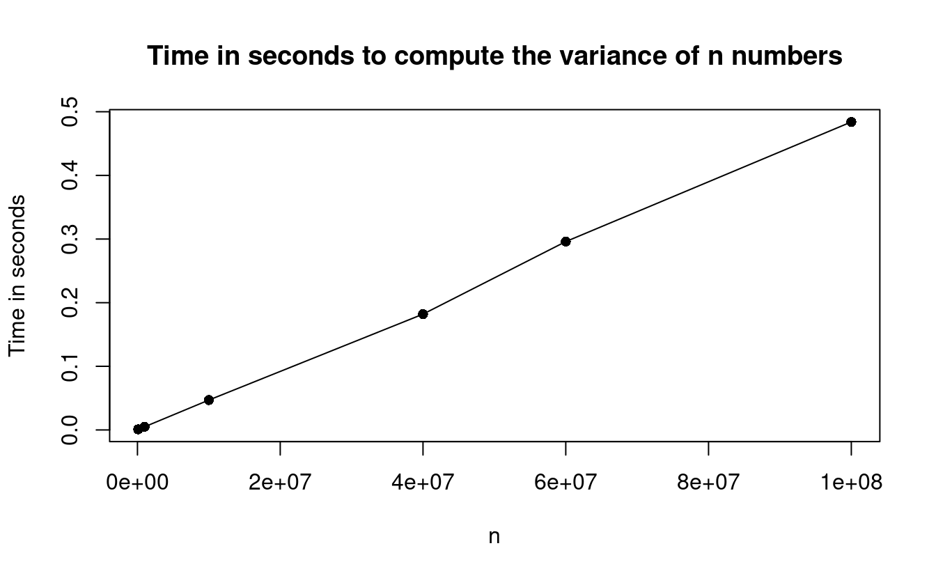
This plot illustrates how the var() function is also a linear time algorithm since it also scales linearly in \(n\).

A tale of two algorithms

Let’s say we want to compute the sum of the squared integers \(1, \dots, n\). Let’s call this output \(a\). Mathematically, this looks like

\[a = 1^{2} + 2^{2} + 3^{2} + \dots + n^{2},\]

which we can write more compactly as

\[a = \sum_{i=1}^{n} i^{2}.\]

How would we do this? If we didn’t know anything about this sum, we might compute \(a\) using the following algorithm, which we’ll call forloopSum since it uses a for loop to sum up the squared integers.

forloopSum <- function(n) {
  sum <- 0
  for (i in 1:n) {
    sum <- sum + i^2
  }
  return(sum)
}

It turns out, however, that there’s actually a formula for computing this so that we don’t need to use a for loop. The formula for this sum is

\[\sum_{i=1}^{n} i^{2} = \frac{n\, (n+1) (2n+1)}{6}.\]

Knowing this formula, we might code up this sum using the following algorithm, which we’ll call formulaSum since it computes this sum directly using the above formula.

formulaSum <- function(n) {
  (n * (n+1) * (2*n+1)) / 6
}

Initial timing comparisons

Let’s compare these two algorithms in R and see the difference in time required.

n <- 1000
forloop.time <- system.time(forloop.ans <- forloopSum(n))
formula.time <- system.time(formula.ans <- formulaSum(n))
c(forloop.time[3], formula.time[3])
#> elapsed elapsed 
#>   0.003   0.000

Keep in mind that timing results can vary widely depending on the computer’s specifications and what else is running at the same time on the computer. If we run the same procedure on the same computer several times in a row, we’re likely to get different timing results unless the procedure finishes almost immediately. Additionally, notice that if a procedure finishes almost immediately (as in our example here), R will frequently show 0 seconds for elapsed time.

Just to be sure that these two computed the same thing, we can also look at the answers we got from the two algorithms.

c(forloop.ans, formula.ans)
#> [1] 333833500 333833500

Good! The two algorithms computed the same answer. (If the two answers didn’t match, we’d know that we coded something wrong somewhere.)

Timing comparisons over a range of values of n

Since computers can square and sum up numbers very, very quickly, let’s again explore some larger values of \(n\) to see if we can see more differences in time required. If we look at values of \(n\) that are very large, however, the answers may be very inaccurate because those squares of large numbers are too large for our computers to represent accurately. In order to compare our solutions accurately, we’ll cap our \(n\) at \(250{,}000\).

Below is some code to run a single experiment across a spread of values of \(n\) ranging from \(100\) to \(250{,}000\). We’ll look at just \(5\) values of \(n\) because we want to be able to see some noticeable timing difference between each value of \(n\).

# Get a range of values of n
nlist <- round(seq(100, 250000, length.out = 5))

# Experiment function
experiment <- function(nlist) {
  
  # Set up output containers
  time1 <- numeric(length=length(nlist))
  time2 <- numeric(length=length(nlist))
  ans1 <- numeric(length=length(nlist))
  ans2 <- numeric(length=length(nlist))
  
  # Run experiment
  for (i in 1:length(nlist)) {
    # Display progress on the console
    cat("integer: ", nlist[i], " ")
    
    # Store time and solutions in our output containers
    time1[i] <- system.time(ans1[i] <- forloopSum(nlist[i]))[3]
    time2[2] <- system.time(ans2[i] <- formulaSum(nlist[i]))[3]
  }
  
  # Return output
  return(list(forloop.time = time1, formula.time = time2, 
              forloop.ans = ans1, formula.ans = ans2))
}

Let’s run our experiment and store it in an object called res. Then let’s compare the solutions we get for each value of \(n\) to make sure that the solutions we get are the same.

res <- experiment(nlist)
#> integer:  100  integer:  62575  integer:  125050  integer:  187525  integer:  250000
res$$forloop.ans - res$$formula.ans
#> [1] 0 0 0 0 0

Let’s also plot the timing results by algorithm. First, we’ll prep the results for use in ggplot2. If you’re unfamiliar with ggplot2, I have a tutorial series on getting started with making data visualizations in R with Part 1, Part 2, and a code lab.

m <- length(nlist)
Method <- c(rep("For Loop", m), rep("Formula", m))
Seconds <- c(res$$forloop.time, res$$formula.time)
n <- rep(nlist, 2)
df <- data.frame(Seconds, Method, n)

Now that our data frame df is ready, let’s make the figure in ggplot2.

library(ggplot2)
ggplot(df, aes(x=n, y=Seconds, color=Method)) +
  geom_line()

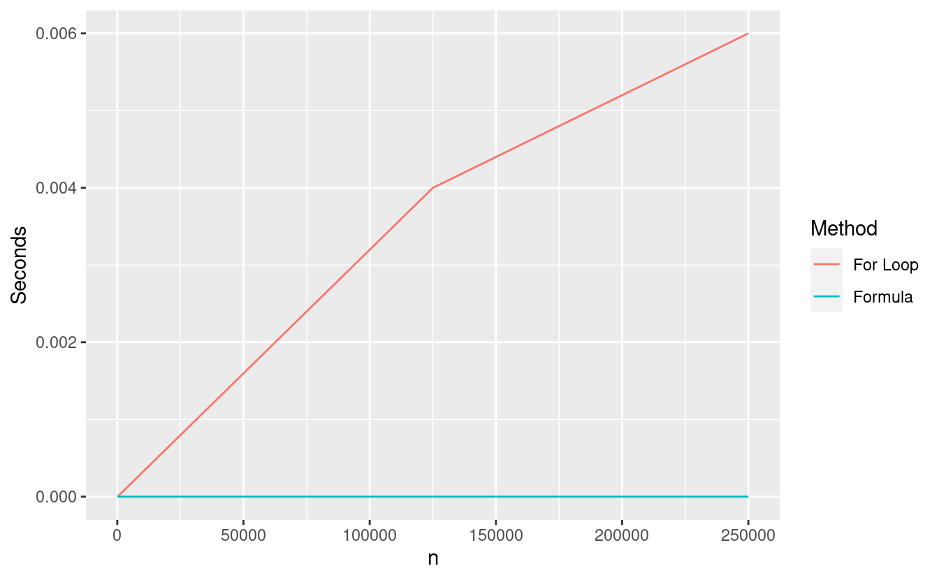
We can see that the formula algorithm finishes immediately regardless of the value of \(n\). This kind of algorithm is called constant time because it is constant with respect to the size of the input data \(n\). This means that the time required to run this algorithm doesn’t depend on \(n\).

By contrast, the forloop algorithm requires linear time since the computational time scales linearly in \(n\). Notice that we might not get a straight line when plotting the time as a function of \(n\) for linear time algorithms in practice. This is because the actual compute time depends on lots of things in your computer, not just on the value of \(n\).

In this simple example, both procedures are very, very fast but by taking larger values of \(n\), we can still start to see some timing differences.

Great job!

In this post, we saw that one aspect of what makes an algorithms better than others is the notion of how the amount of work it requires scales with the size of the input data. We also worked through some simple examples of how much computational work an algorithm requires in terms of basic arithmetic operations, or flops.

We’ve been working with single numbers, or scalars, so far so our algorithms have been very fast. Soon, we’ll move to vectors and matrices and we’ll see some more time-intensive algorithms then.