Getting Started with Linear Algebra in R
So far, we’ve been working with single numbers in our posts. Many kinds of data, however, can be represented by matrices. In order to discuss and learn about methods designed for data stored in matrices, today’s post is a quick tutorial on getting started with linear algebra in R!
If you’re new to linear algebra, this post is for you! We can’t possibly cover everything that you’ll learn in an introductory linear algebra course in this one post. Rather, we’ll just get started with the basic definitions and operations so we can start discussing and working with new methods!
If you’re new to R, I have a two-part series on getting started with coding in R (Part 1 and Part 2). That series will get you up to speed on installing R and RStudio, and the basics of using R so that you can follow along with the code in these posts.
What is a vector?
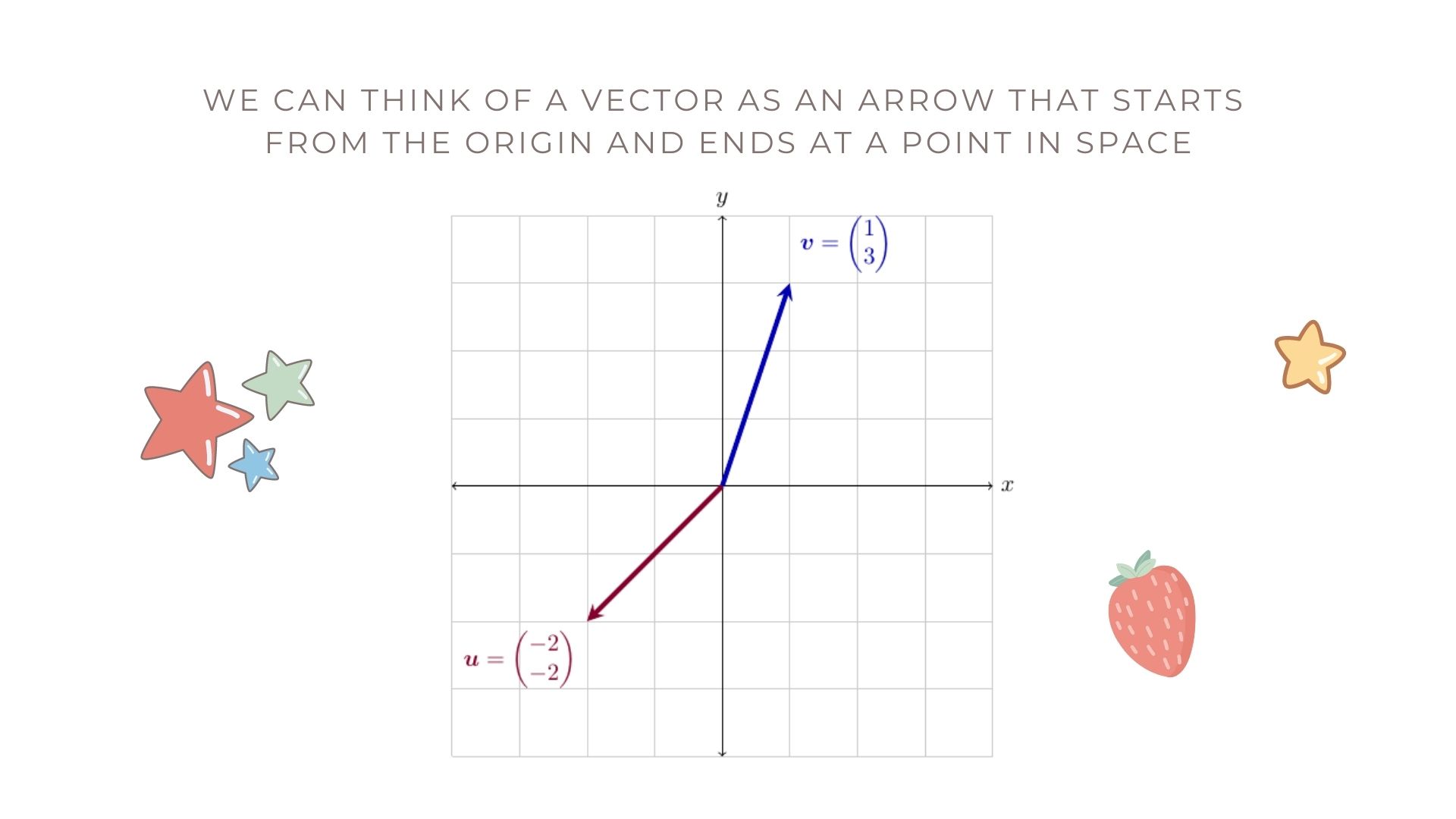
Mechanically, we can think of vectors as an array of numbers, where each slot in the array indicates the value for a different dimension. For example, the following is a two-dimensional vector indicating the coordinates for a point in 2-D space
\[\begin{pmatrix} 1 \\ 3 \end{pmatrix}.\]Geometrically, we can think of vectors as arrows that start at the origin and end at a point in space. For example, below is the vector (we’ll name it \(\mathbf{v}\)) from above in 2-D space. Also pictured is the vector
\[\mathbf{u} = \begin{pmatrix} -2 \\ -2 \end{pmatrix}\]on the same 2-D coordinate system.
Often, we might not specify the actual values of a vector because we’re working generically with any vector in 2-dimensional space. In that case, we would use a variable such as \(\mathbf{x}\) to indicate this vector and we would write \(\mathbf{x} \in \mathbb{R}^{2}\) to indicate that \(\mathbf{x}\) is a 2-dimensional vector whose entries are real numbers. This means that they can take on any value between \(-\infty\) and \(\infty\).
In our posts, we will represent vectors with bold face, lower case letters. If we write \(\mathbf{a} \in \mathbb{R}^{5}\), this means that the vector \(\mathbf{a}\) is a \(5\)-dimensional vector whose entries are real numbers. If we don’t specify the entries in \(\mathbf{a}\), then we indicate its entries with non-bold letters followed by the entry position in subscript
\[\mathbf{a} = \begin{pmatrix} a_{1} \\ a_{2} \\ a_{3} \\ a_{4} \\ a_{5} \end{pmatrix}.\]Throughout our posts, we will always assume that vectors such as \(\mathbf{x}\) and \(\mathbf{a}\) are column vectors as we presented them above. If we want to indicate a row vector, we will specify it with the transpose operation
\[\mathbf{x}^{T} = \begin{pmatrix} 1 & 3 \end{pmatrix}\]and
\[\mathbf{a}^{T} = \begin{pmatrix} a_{1} & a_{2} & a_{3} & a_{4} & a_{5} \end{pmatrix}.\]Sometimes, we may not want to specify the dimension of a vector with an exact value. Rather, we might write \(\mathbf{y} \in \mathbb{R}^{n}\) to indicate the vector \(\mathbf{y}\) contains \(n\) elements whose values are real numbers
\[\mathbf{y} = \begin{pmatrix} y_{1} \\ y_{2} \\ \vdots \\ y_{n} \end{pmatrix}.\]How do we make vectors in R?
In R, there are several ways we can make vectors. Regardless of the method we choose, however, we have to specify the entries. First, we can use the combine function c() to combine several numbers into a vector. We can also use the is.vector() function to find out whether or not R views a particular object as a vector.
If we want to take a sequence of numbers in increments of \(1\) or \(-1\) from some start value to some end value, we can do that using the colon operator : as in the example below.
b <- 1:5
b
#> [1] 1 2 3 4 5
is.vector(b)
#> [1] TRUE
Notice that if we want to increment by \(-1\), we can do that by starting with a larger start number.
b2 <- 9:3
b2
#> [1] 9 8 7 6 5 4 3
is.vector(b2)
#> [1] TRUE
We can also use the colon operator to increment by \(1\) or \(-1\) beginning with non-integer numbers.
b3 <- 0.5:2
b3
#> [1] 0.5 1.5
is.vector(b3)
#> [1] TRUE
If we want to make a vector containing a sequence of numbers that increment based on some value other than \(1\) or \(-1\), we can use the seq() function in R as in the next example.
In the above example, we made a vector that starts at \(1\) and increments by \(2\) until we hit \(10\). In this case, since the next increment of \(2\) above \(9\) would be \(11\), and \(11\) is greater than our end number, the sequence stops at \(9\).
A method we can use to initialize an all-zeros vector of a particular length is the numeric vector function numeric() as in the example below.
We’ll see later that these are all column vectors even though R shows the elements horizontally in the console. To take the transpose of a vector in R, we use the transpose function t() as in the following example.
t(a)
#>      [,1] [,2] [,3] [,4] [,5]
#> [1,]    5    2    7    1    3
t(b)
#>      [,1] [,2] [,3] [,4] [,5]
#> [1,]    1    2    3    4    5
What kinds of mathematical operations can we perform on vectors?
There are a few basic operations we can perform on vectors. In addition to the transpose operation, which we just saw, we can also perform scalar multiplication with vectors. A scalar is just another name for the single numbers that we’ve been mainly working with so far. In our posts, we will indicate scalars by lowercase letters. For example, \(a \in \mathbb{R}\) means that \(a\) is a real-valued scalar, or number.
For a scalar \(a \in \mathbb{R}\) and a vector \(\mathbf{x} \in \mathbb{R}^{n}\), the scalar multiplication operation is performed element-wise on the entries of \(\mathbf{x}\) so that
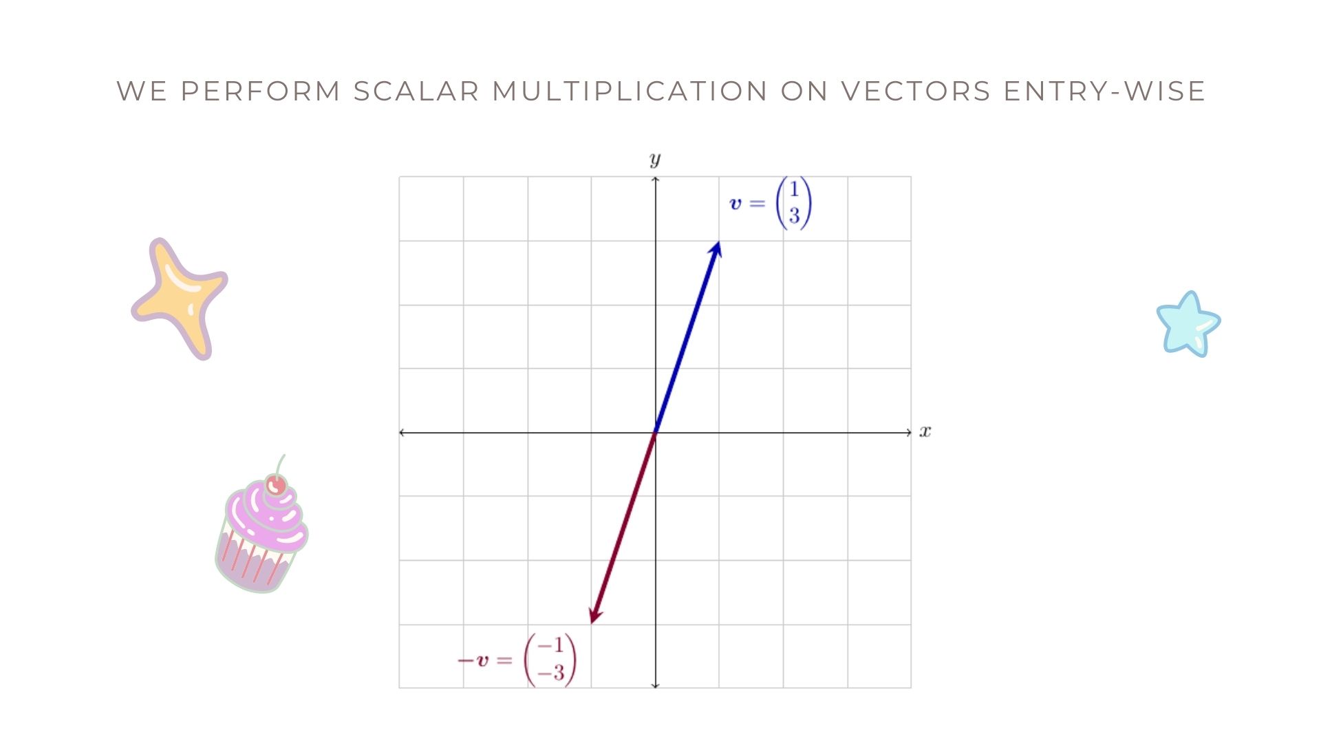
\[a \,\mathbf{x} = a \begin{pmatrix} x_{1} \\ x_{2} \\ \vdots \\ x_{n} \end{pmatrix} = \begin{pmatrix} a \times x_{1} \\ a \times x_{2} \\ \vdots \\ a \times x_{n} \end{pmatrix}.\]Below is a picture of what this looks like in two dimensions! Remember the first vector \(\mathbf{v}\) from above? If we scale it by \(-1\), we get \(-v\) pictured below.
Here’s an example of how to do this in R!
We can also perform addition with vectors of the same size, or dimension. For vectors, the addition operation is also performed element-wise.
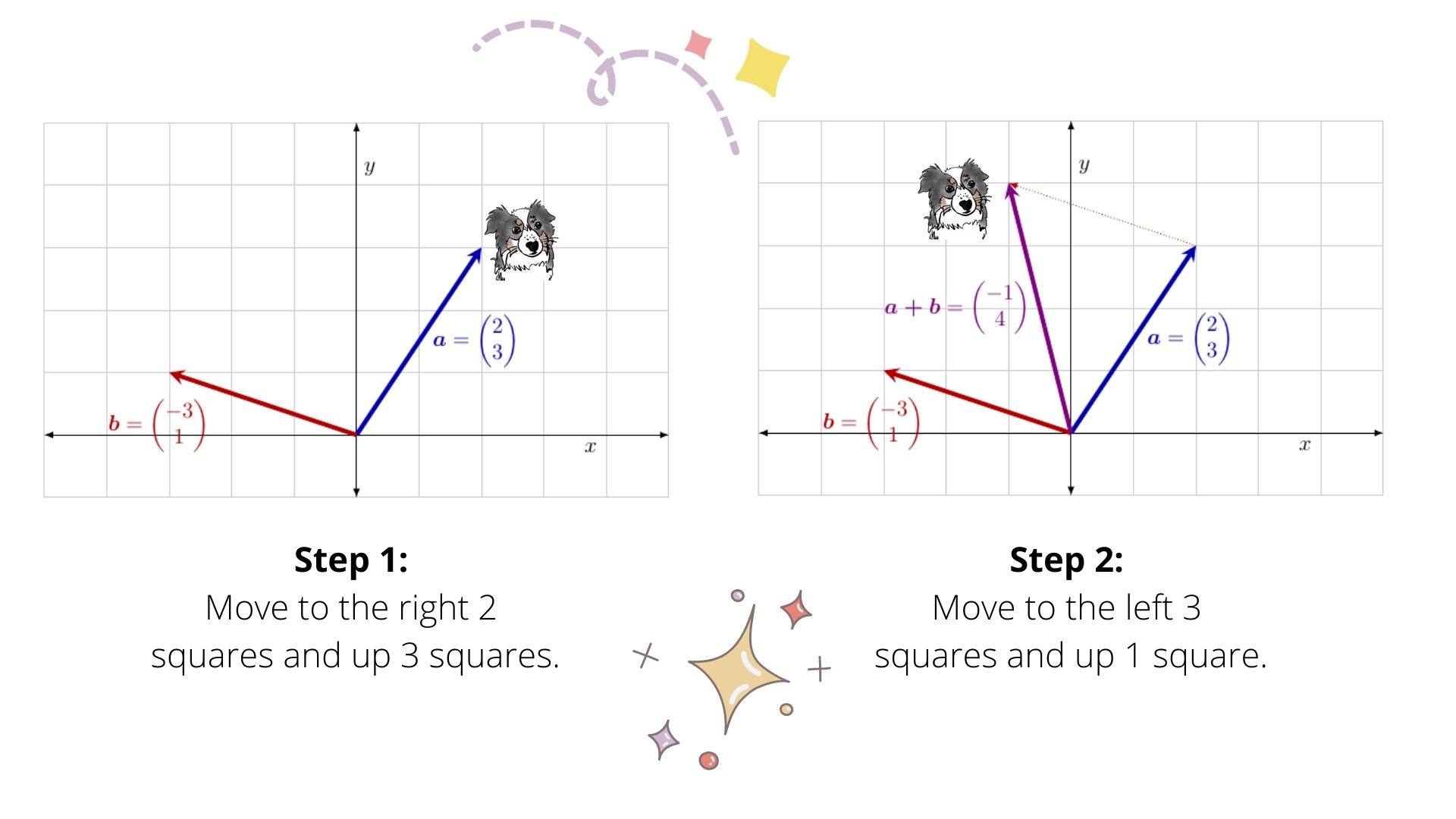
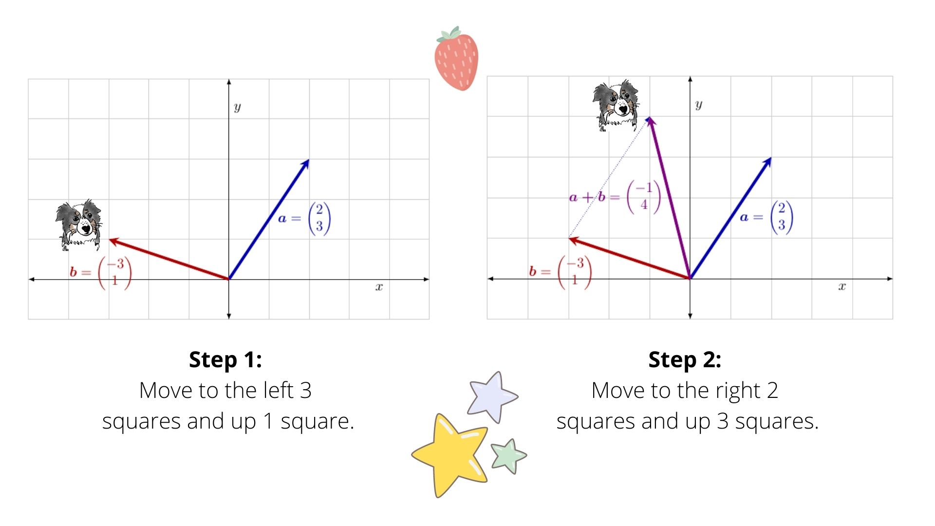
\[\mathbf{x} + \mathbf{y} = \begin{pmatrix} x_{1} \\ x_{2} \\ \vdots \\ x_{n} \end{pmatrix} + \begin{pmatrix} y_{1} \\ y_{2} \\ \vdots \\ y_{n} \end{pmatrix} = \begin{pmatrix} x_{1} + y_{1} \\ x_{2} + y_{2} \\ \vdots \\ x_{n} + y_{n} \end{pmatrix}.\]Here’s a picture of what this looks like in two dimensions! Let’s say we want to add the two vectors \(\mathbf{a}\) and \(\mathbf{b}\) below.
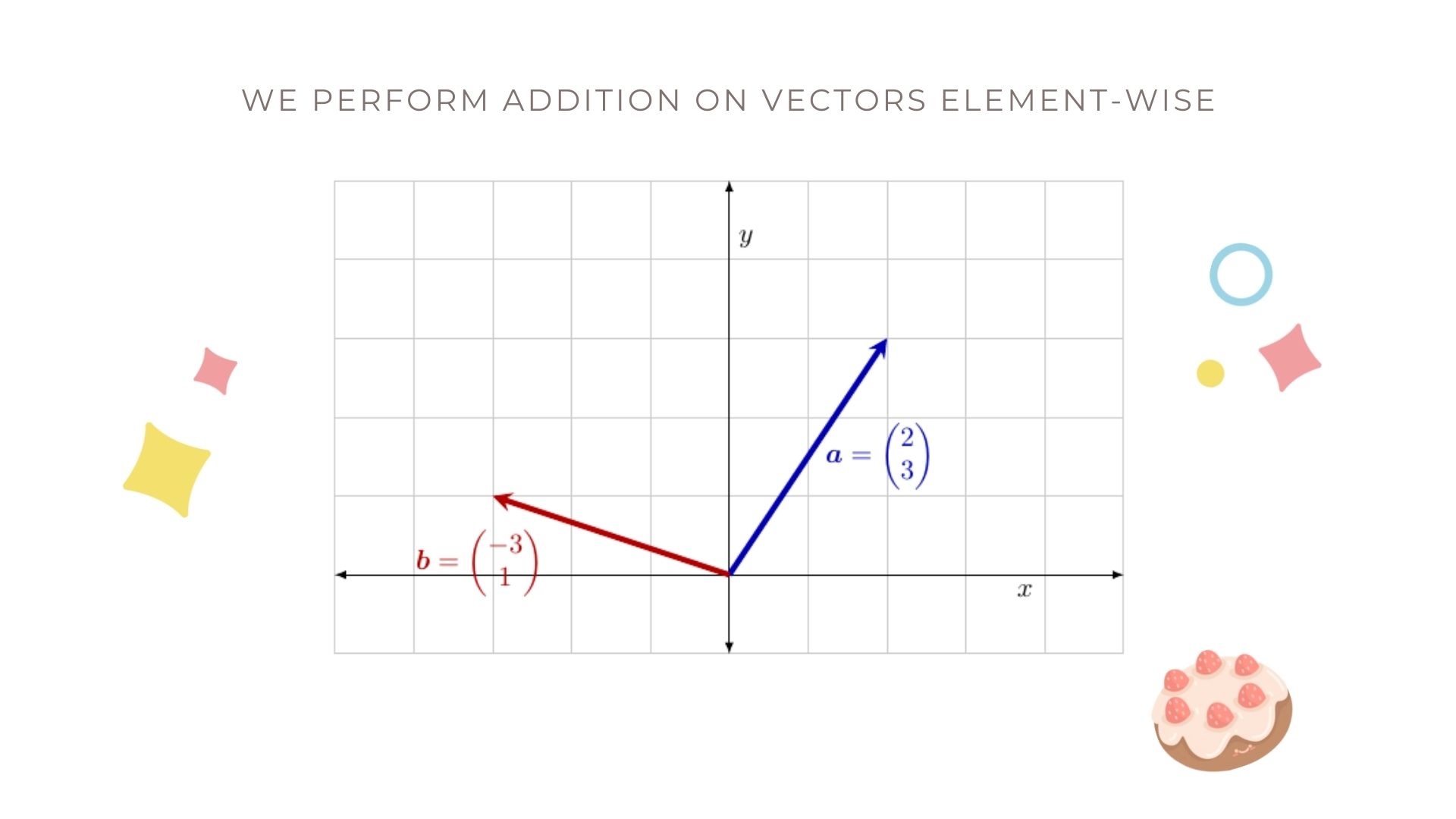
What does this look like in two dimensions? We could start first with \(\mathbf{a}\). The vector \(\mathbf{a}\) says that we move to the right two squares and then up three squares. Once we’re there, the vector \(\mathbf{b}\) says that we move to the left three squares and then up one square.
Alternatively, we would get the same answer if we started first with \(\mathbf{b}\). The vector \(\mathbf{b}\) says that we move to the left three squares and then up one square. Once we’re there, the vector \(\mathbf{a}\) says that we move to the right 2 squares and then up three squares.
Remember that the addition operation includes subtraction since \(\mathbf{x} - \mathbf{y} = \mathbf{x} + (-1)\times\mathbf{y}\). When we combine scalar multiplication and addition, we can get combinations such as the following
\[\frac{1}{a}\, \mathbf{x} + b\, \mathbf{y} = \begin{pmatrix}\frac{1}{a}\, x_{1} \\ \frac{1}{a}\, x_{2} \\ \vdots \\ \frac{1}{a}\, x_{n} \end{pmatrix} + \begin{pmatrix} b\, y_{1} \\ b\, y_{2} \\ \vdots \\ b\, y_{n} \end{pmatrix} = \begin{pmatrix} \frac{1}{a}\, x_{1} + b\, y_{1} \\ \frac{1}{a}\, x_{2} + b\, y_{2} \\ \vdots \\ \frac{1}{a}\, x_{n} + b\, y_{n} \end{pmatrix}.\]Here’s an example of how to do this in R!
a <- 5
x <- 6:-2
b <- 0.5
y <- 1:9
(1/a)*x + b*y
#> [1] 1.7 2.0 2.3 2.6 2.9 3.2 3.5 3.8 4.1
is.vector((1/a)*x + b*y)
#> [1] TRUE
It’s very important to remember that the addition operation only works on vectors of the same length. So if we have \(\mathbf{x} \in \mathbb{R}^{5}\) and \(\mathbf{y} \in \mathbb{R}^{5}\), we can perform the addition operation to get \(\mathbf{x} + \mathbf{y}\). However, if we have \(\mathbf{z} \in \mathbb{R}^{3}\), we cannot add \(\mathbf{z}\) to \(\mathbf{x}\) or to \(\mathbf{y}\) since those pairs of vectors don’t have the same length, or dimension. In this case, we say that their dimensions don’t match.
The inner (or dot) product
There’s another important operation that you can do with vectors of the same dimension. This operation is called the inner product, sometimes also called the dot product. For two column vectors of the same dimension \(\mathbf{x} \in \mathbb{R}^{n}\) and \(\mathbf{y} \in \mathbb{R}^{n}\), this operation can be written in the following three different (but equivalent) ways
\[\langle \mathbf{x}, \mathbf{y} \rangle = \mathbf{x}^{T}\mathbf{y} = \mathbf{x} \cdot \mathbf{y}.\]Regardless of the notation we choose, the inner product operation is the same
\[\mathbf{x}^{T}\mathbf{y} = \begin{pmatrix} x_{1} & x_{2} & \cdots & x_{n} \end{pmatrix} \begin{pmatrix} y_{1} \\ y_{2} \\ \vdots \\ y_{n} \end{pmatrix} = \sum_{i=1}^{n} x_{i}\, y_{i}.\]Do you notice anything unusual about this operation? In previous vector operations, we started with vectors and ended with vectors. The inner product, however, takes in vectors and outputs scalars!
For example, let’s define the following function \(f\) that takes in two vectors and adds them together. We could write it as the following
\[f(\mathbf{x}, \mathbf{y}) = \mathbf{x} + \mathbf{y}.\]Then we would write \(f: \mathbb{R}^{n} \rightarrow \mathbb{R}^{n}\) to indicate that the function \(f\) takes in inputs from \(n\)-dimensional space and maps them to an output in \(n\)-dimensional space.
By contrast, if we write the inner product as the function \(g\) so that
\[g(\mathbf{x}, \mathbf{y}) = \mathbf{x}^{T}\mathbf{y},\]then we would write \(g: \mathbb{R}^{n} \rightarrow \mathbb{R}\) since the function \(g\) takes in inputs from \(n\)-dimensional space and maps them to an output in \(1\)-dimension! In R, we can perform the inner product operation using the transpose function t() followed by the matrix multiplication function %*%.
Length and distance
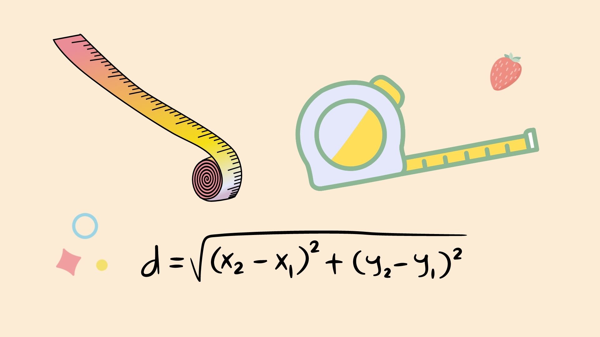
The inner product is closely related to the geometry of vectors. These include our understanding of length, distance, and angles between vectors. We’ll see this more clearly in our next Code Lab, when we use the inner product to make a very simple recommender system.
How is the inner product related to distance? If \(\mathbf{x} = \mathbf{y}\), then the inner product \(\mathbf{x}^{T}\mathbf{x}\) gives us the squared Euclidean norm of the vector \(\mathbf{x}\)! In particular, for any vector \(\mathbf{x} \in \mathbb{R}^{n}\), we define the Euclidean norm, also known as the \(\ell_{2}\)-norm, by
\[\| \mathbf{x} \|_{2} = \sqrt{\mathbf{x}^{T}\mathbf{x}}.\]The Euclidean norm is a standard way of measuring the length of a vector. It is also the standard way of measuring the distance between two vectors, or points, in space.
You might have seen this before in 2- or 3-dimensional space. For any \(\mathbf{x} \in \mathbb{R}^{3}\) and \(\mathbf{y} \in \mathbb{R}^{3}\), the Euclidean distance between \(\mathbf{x}\) and \(\mathbf{y}\) is
\[\text{dist}(\mathbf{x}, \mathbf{y}) = \sqrt{(\mathbf{x} - \mathbf{y})^{T}(\mathbf{x} - \mathbf{y})}.\]This is the Euclidean norm of the vector formed by subtracting \(\mathbf{y}\) from \(\mathbf{x}\)!
What is a matrix?
Now let’s talk about matrices! Initially, we can view a matrix as a two-dimensional array. We will denote matrices by bold-faced capital letters. For example, a matrix \(\mathbf{X} \in \mathbb{R}^{3 \times 4}\) is given by
\[\mathbf{X} = \begin{pmatrix} x_{11} & x_{12} & x_{13} & x_{14} \\ x_{21} & x_{22} & x_{23} & x_{24} \\ x_{31} & x_{32} & x_{33} & x_{34} \end{pmatrix}.\]The entries of a matrix are denoted by non-bold, lower-case letters followed by the row and column indices in subscript.
How do we make matrices in R?
In R, we can make a matrix with the matrix() function. Just as we had to input actual entry values for vectors, we also have to specify the entries of the matrix we want to form.
vec <- 1:12
X <- matrix(vec, nrow=3, ncol=4)
X
#>      [,1] [,2] [,3] [,4]
#> [1,]    1    4    7   10
#> [2,]    2    5    8   11
#> [3,]    3    6    9   12
is.matrix(X)
#> [1] TRUE
In the example above, we told R to form a matrix with 3 rows and 4 columns using the entries in vec. We also stored this matrix as an object named X. Just as we did with vectors, we can use the is.matrix() function to test whether or not R views a particular object as a matrix.
We can see that R filled in the entries of this matrix by columns, moving from left to right. This is the default behavior in R for filling in entries in a matrix. If we look at the documentation for matrix() by typing ?matrix into the console, we’ll find that one of the input options in the matrix() function is the byrow option. If we don’t specify what we want for byrow, the matrix() function will default to setting byrow to FALSE. To fill in the entries by rows instead, we would set byrow=TRUE as in the example below.
Y <- matrix(vec, nrow=3, ncol=4, byrow=TRUE)
Y
#>      [,1] [,2] [,3] [,4]
#> [1,]    1    2    3    4
#> [2,]    5    6    7    8
#> [3,]    9   10   11   12
is.matrix(Y)
#> [1] TRUE
We can also initialize the all zeros matrix in R with the following.
Z <- matrix(0, nrow=5, ncol=3)
Z
#>      [,1] [,2] [,3]
#> [1,]    0    0    0
#> [2,]    0    0    0
#> [3,]    0    0    0
#> [4,]    0    0    0
#> [5,]    0    0    0
is.matrix(Z)
#> [1] TRUE
What kinds of operations can we perform on matrices?
Similar to vectors, we can perform scalar multiplication and addition with matrices of the same dimensions. Also similar to vectors, the scalar multiplication and addition operations occur element-wise on matrices.
For example, if we have a scalar \(a \in \mathbb{R}\) and matrices \(\mathbf{X}\in \mathbb{R}^{2 \times 3}\) and \(\mathbf{Y} \in \mathbb{R}^{2 \times 3}\), then
\[a\, \mathbf{X} + \mathbf{Y} = a \begin{pmatrix} x_{11} & x_{12} & x_{13} \\ x_{21} & x_{22} & x_{23} \end{pmatrix} + \begin{pmatrix} y_{11} & y_{12} & y_{13} \\ y_{21} & y_{22} & y_{23} \end{pmatrix} = \begin{pmatrix} a\, x_{11} + y_{11} & a\, x_{12} + y_{12} & a\, x_{13} + y_{13} \\ a\, x_{21} + y_{21} & a\, x_{22} + y_{22} & a\, x_{23} + y_{23} \end{pmatrix}.\]Let’s see an example of this in R so that we can verify that the entries of the sum \(a\mathbf{X} + \mathbf{Y}\) are what we expect! First, we’ll form the objects a, X, and Y.
a <- 10
vec <- 1:6
X <- matrix(vec, nrow=2, ncol=3)
X
#>      [,1] [,2] [,3]
#> [1,]    1    3    5
#> [2,]    2    4    6
Y <- matrix(vec, nrow=2, ncol=3, byrow=TRUE)
Y
#>      [,1] [,2] [,3]
#> [1,]    1    2    3
#> [2,]    4    5    6
Then let’s perform the scalar multiplication and addition in R and verify that the entries are what we’d expect!
a * X +  Y
#>      [,1] [,2] [,3]
#> [1,]   11   32   53
#> [2,]   24   45   66
Is this the same answer you got when you computed \(a\, \mathbf{X} + \mathbf{Y}\)?
Matrix-vector multiplication
One of the most fundamental matrix operations we can perform is matrix-vector multiplication. For a matrix \(\mathbf{A} \in \mathbb{R}^{2 \times 3}\) and a vector \(\mathbf{v} \in \mathbb{R}^{3}\), we have
\[\mathbf{A}\mathbf{v} = \begin{pmatrix} a_{11} & a_{12} & a_{13} \\ a_{21} & a_{22} & a_{23} \end{pmatrix} \begin{pmatrix} v_{1} \\ v_{2} \\ v_{3} \end{pmatrix} = v_{1}\begin{pmatrix} a_{11} \\ a_{21}\end{pmatrix} + v_{2}\begin{pmatrix} a_{12} \\ a_{22}\end{pmatrix} + v_{3}\begin{pmatrix} a_{13} \\ a_{23}\end{pmatrix}.\]So we see that matrix-vector multiplication between \(\mathbf{A}\) and \(\mathbf{v}\) results in a weighted sum of the columns of \(\mathbf{A}\), where the weights are the corresponding entries in \(\mathbf{v}\).
A few things to keep in mind…
-
In order for matrix-vector multiplication to occur, the dimensions between the matrix and the vector have to match! Specifically, the vector \(\mathbf{v}\) must have the same dimension as the second dimension (the number of columns) in \(\mathbf{A}\)!
-
We can view the matrix \(\mathbf{A}\) as a linear operator, or linear function, that takes in vectors in \(\mathbf{R}^{3}\) and outputs vectors in \(\mathbf{R}^{2}\)! This is also the first dimension (the number of rows) in \(\mathbf{A}\).
Let’s see an example of this in R!
vec <- 2*1:6
A <- matrix(vec, nrow=2, ncol=3)
A
#>      [,1] [,2] [,3]
#> [1,]    2    6   10
#> [2,]    4    8   12
v <- rep(0.5, 3)
v
#> [1] 0.5 0.5 0.5
is.vector(v)
#> [1] TRUE
Here, we’ve formed a matrix \(\mathbf{A} \in \mathbb{R}^{2 \times 3}\) and a vector \(\mathbf{v} \in \mathbb{R}^{3}\). We’ve also used a new method to form this vector! We used the rep() function to form a vector of length \(3\) whose entries are all \(0.5\).
Now we can perform the matrix-vector multiplication with the matrix multiplication function %*%.
A %*% v
#>      [,1]
#> [1,]    9
#> [2,]   12
We see that the matrix-vector product \(\mathbf{Av} \in \mathbb{R}^{2}\), just as we worked out previously. We also see that the product is the sum of \(0.5\) times each of the columns in \(\mathbf{A}\).
as.matrix(v[1] * A[,1] + v[2] * A[,2] + v[3] * A[,3])
#>      [,1]
#> [1,]    9
#> [2,]   12
In the example above, I’ve added the as.matrix() wrapper function so that the weighted sum of the columns appears as a column vector in the console. This is because (as we mentioned earlier) R displays the entries of vectors horizontally in the console even though it recognizes them as column vectors.
Another look at matrix-vector multiplication
Algebraically, matrix-vector multiplication between a matrix \(\mathbf{A}\) and a vector \(\mathbf{v}\) can also be viewed as the inner products between the rows of \(\mathbf{A}\) and the the vector \(\mathbf{v}\). Specifically, let \(\mathbf{A}_{(1,:)}\) and \(\mathbf{A}_{(2,:)}\) be column vectors that form the first and second rows of \(\mathbf{A}\). Then the matrix-vector product \(\mathbf{Av}\) can also be written as
\[\mathbf{A}\mathbf{v} = \begin{pmatrix} a_{11} & a_{12} & a_{13} \\ a_{21} & a_{22} & a_{23} \end{pmatrix} \begin{pmatrix} v_{1} \\ v_{2} \\ v_{3} \end{pmatrix} = \begin{pmatrix} \langle \mathbf{A}_{(1,:)}, \mathbf{v} \rangle \\ \langle \mathbf{A}_{(2,:)}, \mathbf{v} \rangle \end{pmatrix}.\]Matrix-matrix multiplication
Now that we’re comfortable with matrix-vector multiplication, we can easily extend this idea to matrix-matrix multiplication! Say we have two matrices \(\mathbf{A} \in \mathbb{R}^{3 \times 2}\) and \(\mathbf{B} \in \mathbb{R}^{2 \times 2}\). We obtain the matrix product \(\mathbf{AB}\) as follows
\[\mathbf{AB} = \begin{pmatrix} a_{11} & a_{12} \\ a_{21} & a_{22} \\ a_{31} & a_{32} \end{pmatrix} \begin{pmatrix} b_{11} & b_{12} \\ b_{21} & b_{22} \end{pmatrix} = \begin{bmatrix} b_{11} \begin{pmatrix} a_{11} \\ a_{21} \\ a_{31} \end{pmatrix} + b_{21} \begin{pmatrix} a_{12} \\ a_{22} \\ a_{32} \end{pmatrix} & b_{12} \begin{pmatrix} a_{11} \\ a_{21} \\ a_{31} \end{pmatrix} + b_{22} \begin{pmatrix} a_{12} \\ a_{22} \\ a_{32} \end{pmatrix} \end{bmatrix}.\]A few things to keep in mind…
-
The first column of \(\mathbf{AB}\) is the matrix-vector product between \(\mathbf{A}\) and the first column of \(\mathbf{B}\). Similarly, the second column of \(\mathbf{AB}\) is the matrix-vector product between \(\mathbf{A}\) and the second column of \(\mathbf{B}\). We see that matrix-matrix multiplication is the result of matrix-vector multiplication between \(\mathbf{A}\) and the columns of \(\mathbf{B}\)!
-
The dimensions have to match! Just as the dimension of the vector has to match the number of columns of the matrix in matrix-vector multiplication, so the number of rows in \(\mathbf{B}\) has to match the number of columns in \(\mathbf{A}\).
In R, we can perform matrix-matrix multiplication with the %*% function.
A <- matrix(vec, nrow=3, ncol=2)
A
#>      [,1] [,2]
#> [1,]    2    8
#> [2,]    4   10
#> [3,]    6   12
B <- matrix(c(0.5, -0.5, 2, 1), nrow=2, ncol=2)
B
#>      [,1] [,2]
#> [1,]  0.5    2
#> [2,] -0.5    1
A %*% B
#>      [,1] [,2]
#> [1,]   -3   12
#> [2,]   -3   18
#> [3,]   -3   24
Great job!

In this post, we discussed the basics of what vectors and matrices are, how to make them in R, and the basic mathematical operations you can perform on them. In our next Code Lab, we’ll get more practice working with vector operations in R and also develop our understanding of distance and angles between vectors by building a simple recommender system in R!


