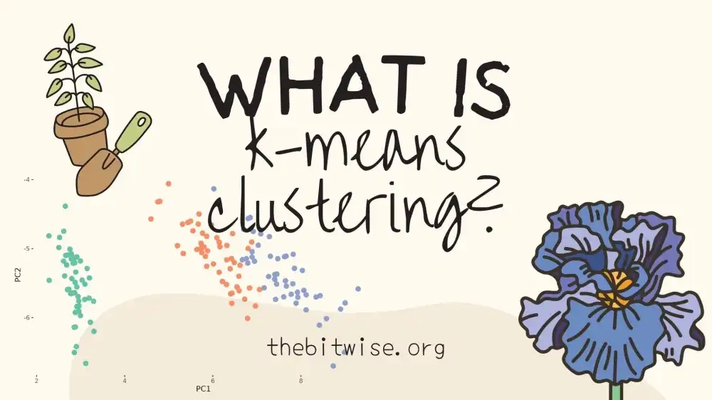
What is k-means Clustering?
In previous posts, we discussed vectors and vector norms in a basic introduction to linear algebra and got some practice working with them in our Code Lab on coding a simple recommendation system in R. Today, we’ll follow up on those skills and take a first look at k-means clustering, a machine learning algorithm for clustering!
The goal of k-means clustering is to assign observations to different groups (or classes) when we don’t know their actual group membership labels. Methods for assigning observations to groups without membership labels are also known as unsupervised learning methods since they’re not supervised, or aided, by existing membership information. Since it’s a relatively simple algorithm and quite effective in many situations, k-means clustering has been widely used in numerous applications and there are many variations on it. Today, we’ll study and implement a version called Lloyd’s algorithm.
As we’ve done in our previous posts, we’ll be coding in R. If you’re new to R, I have a tutorial on getting started with coding in R in a two-part series here and here. This series will get you up to speed on installing and using R and RStudio so you can follow along with this post.
What is k-means clustering?
Let’s say that we have \(n\) observations with \(p\) measurements on each observation. For example, if the observations are patients in a hospital, their measurements might include things like their age, height, weight, and many other diagnosis or treatment measurements at a particular point in time. Let’s represent the observations as \(p\)-dimensional vectors
\[\boldsymbol{x}_{i} \in \mathbb{R}^{p} \quad \text{for} \quad i=1, 2, 3, \dots, n.\]If you’re new to the \(\mathbb{R}^{p}\) notation, this just means that each \(\boldsymbol{x}_{i}\) is a vector containing \(p\) entries
\[\boldsymbol{x}_{i} = \begin{pmatrix}x_{i1} \\ x_{i2} \\ x_{i3} \\ \vdots \\ x_{ip} \end{pmatrix},\]where each entry contains a real number. Each of these \(n\) vectors is a point in \(\mathbb{R}^{p}\).
What is the goal of k-means clustering?

The goal of k-means clustering is to place these \(n\) points into \(k\) groups in such a way that points in the same group are close together. To measure the distance between two points, we’ll use the Euclidean distance that we discussed in our basic introduction to linear algebra.
How does k-means clustering work?
How do we make sure that points in the same group are close together while points in different groups are far apart? This is where the means in k-means comes in! The means refer to the group centroids, which are computed as the mean of all the points in the group. Since there are \(k\) groups, we have \(k\) group centroids.
Let’s denote the groups with \(G_{1}, G_{2}, ..., G_{k}\). Each group is a set containing the points that belong to it. Let’s also denote the group centroids with \(\boldsymbol{\mu}_{1}, \boldsymbol{\mu}_{2}, \dots, \boldsymbol{\mu}_{k}\). The lowercase Greek letter \(\mu\) (pronounced like “mew”) is frequently used to denote means and we will use boldface font to indicate that they are vectors. Since vector means are computed element-wise on the entries, the group means are also points in \(\mathbb{R}^{p}\).
Mathematically, we can write the k-means problem as
\[\min_{\boldsymbol{\mu}_{1}, \boldsymbol{\mu}_{2}, \dots, \boldsymbol{\mu}_{k}, G_{1}, G_{2}, \dots, G_{k}} \sum_{j=1}^{k} \sum_{\boldsymbol{x}\in G_{j}} \|\boldsymbol{x} - \boldsymbol{\mu}_{j}\|^{2}_{2}.\]This means that for the \(j^{th}\) group \(G_{j}\) (recall that \(j\) begins with \(1\) and goes up to \(k\)), we will sum the squared Euclidean distance between all the points \(\boldsymbol{x}\) in the group and the \(j^{th}\) group centroid \(\boldsymbol{\mu}_{j}\). This is indicated by \(\sum_{\boldsymbol{x}\in G_{j}} \|\boldsymbol{x}- \boldsymbol{\mu}_{k}\|^{2}_{2}\). Then we will sum the sums from all the groups. We will return the centroids (the \(\boldsymbol{\mu}_{j}\) for \(1\le j\le k\)) and groups (the \(G_{j}\) for \(1 \le j \le k\)) that minimize this sum of sums.
What is the k-means algorithm?
Now that we know what k-means clustering does, let’s look at how we can compute it! Lloyd’s algorithm for k-means clustering does this with the following steps.
- Initalize the centroids \(\boldsymbol{\mu}_{1}, \boldsymbol{\mu}_{2}, \dots, \boldsymbol{\mu}_{k}\).
- For each of the \(n\) observations, compute the Euclidean distance between the observation and each of the \(k\) group centroids. Assign each observation to the group with the closest group centroid.
- Update the centroids with the new group means.
Notice that in Step 1, we have to initialize the centroids because we don’t know which observations belong to which groups. In practice, some initializations are better than others. We will start by randomly selecting \(k\) observations from our \(\boldsymbol{x}_{i}\) as our initializations.
Also notice that in Step 3, our new mean update also solves our minimization problem
\[\boldsymbol{\mu}_{j} \leftarrow \arg \min_{\boldsymbol{\mu}} \sum_{\boldsymbol{x}\in G_{j}} \|\boldsymbol{x} - \boldsymbol{\mu}\|^{2}_{2} = \frac{1}{|G_{j}|} \sum_{\boldsymbol{x} \in G_{j}} \boldsymbol{x},\]where \(\vert G_{j}\vert\) denotes the size, or number of objects, in the \(j^{th}\) group.
We’ll repeat the last 2 steps until we attain our chosen maximum number of iterations or until the centroids stop changing. Now that we know an algorithm for k-means clustering, we can implement it in R!
Implementing k-means clustering in R
Let’s implement k-means clustering in R by turning the steps we just described into code! To help us do this, let’s first load a real dataset so that we can work through the steps in R.
Loading the iris dataset

We’ll be working with Edgar Anderson’s iris dataset, which was published in 1936 and has been widely used to demonstrate clustering and classification machine learning methods. The dataset contains \(n=150\) flowers from \(k=3\) different iris species (setosa, versicolor, and virginica).

There are \(p=4\) measurements (in cm) on each flower: sepal length, sepal width, petal legnth, and petal width.

This dataset is great for demonstrating k-means clustering because the group sizes are equal; each group contains \(50\) flowers. The iris dataset comes preloaded in R in the datasets package. So we can read the documentation on it right away with the ? function.
?irisTo load the dataset into our environment, we can use the data() function.
data(iris)Let’s take a look at the first few entries in the dataset with the head() function.
head(iris)
#>   Sepal.Length Sepal.Width Petal.Length Petal.Width Species
#> 1          5.1         3.5          1.4         0.2  setosa
#> 2          4.9         3.0          1.4         0.2  setosa
#> 3          4.7         3.2          1.3         0.2  setosa
#> 4          4.6         3.1          1.5         0.2  setosa
#> 5          5.0         3.6          1.4         0.2  setosa
#> 6          5.4         3.9          1.7         0.4  setosa
We see that the observations are contained on the rows while the variables, or measurements, are contained on the columns. The first four columns contain the \(p=4\) measurements that we want to use to predict group assignment so let’s subset our data for the \(4\) columns and name our data matrix \(\boldsymbol{X}\).
X <- as.matrix(iris[,1:4])The fifth column contains the group labels. Although our k-means clustering algorithm does not employ the labels, it’s nice that we have them for this particular dataset so we can compare the group assignments we’ll obtain later.
Each observation, or point, in the iris dataset has \(4\) dimensions so we can’t plot these points directly. However, we can use a dimension reduction technique called principal components analysis to represent the points in \(2\) dimensions. We’ll walk through the details of principal components analysis in a future post so we won’t discuss how we performed the dimension reduction for now. Below is a plot of the first two principal components (a 2-D representation) of the iris data. Each point represents a flower from the dataset and the coloring indicates the species.

The plot shows us that flowers in the same species appear to cluster together in the first two principal components. It’s great when we know the group memberships ahead of time but what if we don’t have that information? This is where k-means clustering can be very useful! Let’s get started with implementing k-means clustering in R!
Step 1: Initialize the centroids
First, we’ll initialize the \(k\) centroids by randomly selecting \(k\) observations from our \(\boldsymbol{x}_{i}\). To randomly select \(k\) observations without replacement from the numbers \(1, 2, \dots, n\), we can use the sample() function. We can view the documentation for the sample() function with ?sample. From the documentation, we can see that the function defaults to sampling with replacement since it automatically sets replace=FALSE.
# Identify the number of observations n and number of groups k
n <- nrow(X)
k <- length(unique(y))

# Randomly select k integers from 1 to n (without replacement)
selects <- sample(1:n, k)
selects # to view the selected observations
#> [1] 128  84  20

# Initialize the centroids with the selected observations
centroids <- X[selects,]
centroids # to view the initial centroids
#>      Sepal.Length Sepal.Width Petal.Length Petal.Width
#> [1,]          6.1         3.0          4.9         1.8
#> [2,]          6.0         2.7          5.1         1.6
#> [3,]          5.1         3.8          1.5         0.3
Let’s plot the observations and take a look at the centroids we randomly selected! The figure below shows a plot of the first two principal components of the data with the randomly selected centroids colored in orange.

To keep things simple, let’s assume that the centroids are listed in order so that the \(j^{th}\) row in centroids contains the centroid for the \(j^{th}\) group.
Step 2: Assign each point to the group with the closest centroid
Next, we’ll first compute the Euclidean distance between each point and each centroid. Since we don’t need to store these distances, let’s just write a function that computes the distance between a single point and the \(k\) centroids, and returns the group with the smallest distance.
There are many ways we can write this function. In the version we’ll code together here, our function will take in two inputs: 1) a point and 2) our centroids matrix from above. Our output will be the group number of the closest centroid. Inside the function, we’ll initialize a container for storing the computed distances, we’ll use a forloop to iterate through the \(k\) centroids, and we’ll use the which.min() function to identify the index of the closest centroid.
Recall from our basic introduction to linear algebra that we can compute the Euclidean distance between two points \(\boldsymbol{a}\) and \(\boldsymbol{b}\) of the same length with the following square root of an inner product
\[\text{dist}(\boldsymbol{a}, \boldsymbol{b}) = \sqrt{(\boldsymbol{a} - \boldsymbol{b})^{T} (\boldsymbol{a} - \boldsymbol{b})}.\]Since our output (the centroid with minimum Euclidean distance) remains unchanged if we use the squared Euclidean distance instead, we’ll do that since we can save a tiny bit of time by not having to compute the square root.
dist_to_centroids <- function(point, centroids) {

  # Initialize distance container
  k <- nrow(centroids)
  dist <- numeric(length=k)

  # Compute squared Euclidean distance to each centroid
  for (a in 1:k) {
    diff <- point - centroids[a,]
    dist[a] <- t(diff) %*% diff
  }

  # Return closest centroid
  return(which.min(dist))
}
We can test our function with the first observation in our data. Notice that our original group labels are the species names while the dist_to_centroids() function returns the index number of the closest centroid. That’s okay because we’re just interested in assigning points to groups right now; we’re not concerned with the actual group names at this point.
dist_to_centroids(X[1,], centroids)
#> [1] 3
Now we can use our dist_to_centroids() function to assign each of the points to the group with the closest centroid. To do this, we’ll initialize a container for storing the group assignments.
# Initialize container for storing group assignments
n <- nrow(X)
groups <- numeric(length=n)

# Assign each point to the group with closet centroid
for (b in 1:n) {
  groups[b] <- dist_to_centroids(X[b,], centroids)
}
Let’s take a look at our current group assignments!
groups
#>   [1] 3 3 3 3 3 3 3 3 3 3 3 3 3 3 3 3 3 3 3 3 3 3 3 3 3 3 3 3 3 3 3 3 3 3 3 3 3
#>  [38] 3 3 3 3 3 3 3 3 3 3 3 3 3 1 1 1 2 1 2 1 2 1 1 2 1 2 1 1 1 1 2 2 2 1 1 2 2
#>  [75] 1 1 1 1 1 1 2 2 1 2 1 1 1 2 1 2 2 1 2 2 2 1 1 1 3 1 1 2 1 2 1 2 2 2 2 1 1
#> [112] 2 1 2 1 1 1 1 2 2 1 1 2 1 1 1 1 1 2 2 2 1 1 2 2 1 1 1 1 1 1 1 2 1 1 1 2 1
#> [149] 1 1
In the figure below, we show the initial assignments on the points by their coloring. We also show the centroids that gave rise to the current assignments in black.

It’s okay if many points are initially assigned to the same group since initial clustering assignments will depend on the random centroid initialization. This is fine because we’re going to update the centroids and then repeat Steps 2 and 3 until the centroids stop changing so our final assignments can look substantially different.
Step 3: Update the centroids
Our last step is to update the centroids. To do that, we’ll first use the which() function to identify the points belonging to each group. In code chunk below, we’ll use the apply() function to apply the mean() function to each of the columns of the rows subset from \(\boldsymbol{X}\). We update the centroids by storing the computed means in the respective rows of centroids.
# Save current centroids before updating for testing convergence later
previous_centroids <- centroids

groupLabels <- unique(groups)
for (c in 1:k) {
  centroids[c,] <- apply(X[which(groups==groupLabels[c]), ], 2, mean)
}
Let’s take a look at our new centroids!
centroids # look at centroids
#>      Sepal.Length Sepal.Width Petal.Length Petal.Width
#> [1,]     5.007843    3.409804     1.492157   0.2627451
#> [2,]     6.382258    3.053226     4.970968   1.7822581
#> [3,]     6.091892    2.578378     4.848649   1.5135135
Now let’s look at the same plot from before with the updated centroids!

Stopping criteria
We’ll continue looping over Steps 2 and 3 until one of two things occurs. Either we complete a preset maximum number of iterations, or completed loops, or the centroids stop changing when we update them in Step 3.
To find out when the centroids stop changing, we’ll compute the Euclidean distance between the updated centroids and the previous ones for each group. If the updated centroids are exactly the same as the previous ones, then the distance between them will be \(0\).
Let’s try this out and compute the distance between the updated centroids and the previous ones! We use the Frobenius matrix norm with the norm() function below. This is the same as stringing the entries of the matrix together into a really long vector and then computing the vector Euclidean norm.
norm(centroids - previous_centroids, "F")
#> [1] 5.551605
In practice, we may not need to continue looping until the distance between the current and next centroid for each group is exactly \(0\). Instead, it’s usually enough if they’re very close to each other. It’s up to the user to decide how close is close enough so we refer to this as a convergence tolerance and we’ll stop looping when the distance between the updated centroid and the previous one for each group is within a predefined tolerance level.
Putting the steps together into a function for k-means clustering
Now let’s combine all the steps and the stopping criteria together into a single function for performing k-means clustering!
For our inputs, we’ll include the following:
X- Our data in matrix formk- The number of intended clustersmaxiters- The maximum number of iterationstol- The convergence toleranceseed- Seed for random centroid initialization
Let’s set the default maximum number of iterations to \(100\) and the default convergence tolerance to \(1^{-4}\). Also recall that in Step 2, we use the dist_to_centroids() function we made above so the function below won’t run without the dist_to_centroids() function.
The only thing that we really need to output from this function is the final group assignment. However, there are a couple of other items that we might want to output for sanity checks. The version below includes some of those in the output.
kmeans <- function(X, k, maxiters=100, tol=1e-4, seed=123) {

  # -----------------------------------
  # Step 1: Initialize centroids
  # -----------------------------------

  # Identify the number of observations n
  n <- nrow(X)

  # Randomly select k integers from 1 to n (without replacement)
  set.seed(seed)
  selects <- sample(1:n, k)
  selects # to view the selected observations

  # Initialize the centroids with the selected observations
  centroids <- X[selects,]
  centroids # to view the initial centroids

  # Initialize a container for checking the convergence progress
  diff <- numeric(length=maxiters)

  for (a in 1:maxiters) {
    # -----------------------------------------
    # Step 2: Assign observations to clusters
    # -----------------------------------------

    # Initialize container for storing group assignments
    groups <- numeric(length=n)

    # Assign each point to the group with closet centroid
    for (b in 1:n) {
      groups[b] <- dist_to_centroids(X[b,], centroids)
    }

    # -----------------------------------------
    # Step 3: Update centroids
    # -----------------------------------------

    # Save current centroids
    previous_centroids <- centroids

    groupLabels <- unique(groups)
    for (c in 1:k) {
      centroids[c,] <- apply(X[which(groups==groupLabels[c]), ], 2, mean)
    }

    # -----------------------------------------
    # Check for convergence
    # -----------------------------------------

    diff[a] <- norm(centroids - previous_centroids, "F")
    if (diff[a] < tol) {
      diff <- diff[1:a]
      break
    }

  }

  # Return group assignments
  return(list(groups=groups, iters=a, diff=diff, centroids=centroids))
}
Let’s try out our function!
result <- kmeans(X, 3)
result
#> $$groups
#>   [1] 1 1 1 1 1 1 1 1 1 1 1 1 1 1 1 1 1 1 1 1 1 1 1 1 1 1 1 1 1 1 1 1 1 1 1 1 1
#>  [38] 1 1 1 1 1 1 1 1 1 1 1 1 1 2 3 2 3 3 3 3 3 3 3 3 3 3 3 3 3 3 3 3 3 3 3 3 3
#>  [75] 3 3 3 2 3 3 3 3 3 3 3 3 3 3 3 3 3 3 3 3 3 3 3 3 3 3 2 3 2 2 2 2 3 2 2 2 2
#> [112] 2 2 3 3 2 2 2 2 3 2 3 2 3 2 2 3 3 2 2 2 2 2 3 2 2 2 2 3 2 2 2 3 2 2 2 3 2
#> [149] 2 3
#>
#> $$iters
#> [1] 15
#>
#> $$diff
#>  [1] 2.76205257 1.81166732 0.65871408 3.37310255 0.47984871 0.25179622
#>  [7] 0.11155094 0.10240597 0.12418090 0.09713929 0.10867737 0.07687992
#> [13] 0.08340425 0.03815921 0.00000000
#>
#> $$centroids
#>      Sepal.Length Sepal.Width Petal.Length Petal.Width
#> [1,]     5.006000    3.428000     1.462000    0.246000
#> [2,]     6.853846    3.076923     5.715385    2.053846
#> [3,]     5.883607    2.740984     4.388525    1.434426
The figure below shows the observations colored according to their final group assignments and the final group centroids in black.

Notice that the coloring of the points may be different we expect but we’re not too concerned about this since we can always recolor the groups by changing the label names or telling R to plot them in a different order.
Thinking about our results…
Notice that our k-means clustering function returns numeric labels rather than the species names. If we want, we can also go back to match the group numbers to the species names! Do you have ideas about how you could do this?
Now we can visually compare the figure of our clustering assignments from our k-means clustering algorithm with the one we got previously with the species labels. Can you tell which points were misclassified with k-means clustering? Why do you think they were misclassfied?
Great job!

In this post, we discussed k-means clustering: its objective, how it works, and the steps in the variant of it from Lloyd’s algorithm. Then we implemented k-means clustering in R and tried it out on the famous iris dataset! Great job!
Photo Credits: Iris setosa, versicolor, and virginica images by anonymous contributor, D. Gordon E. Robertson, and Eric Hunt, Wikimedia Commons.