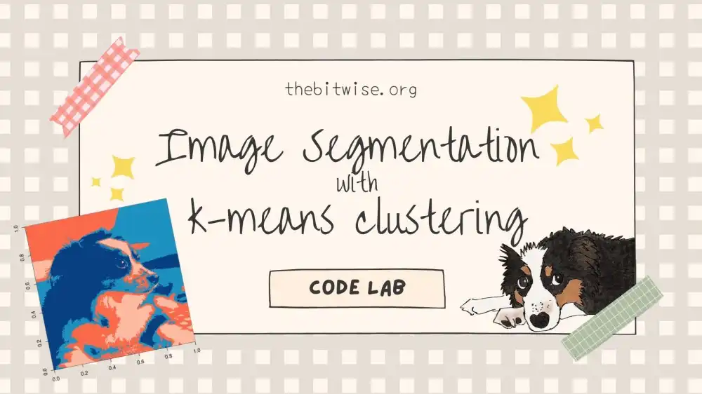
Image Segmentation with k-means Clustering
In our last post, we implemented our own k-means clustering algorithm in R! Today, we’ll explore k-means clustering some more with a Code Lab to see how we can use the algorithm we coded up last time to cluster pixels in an image!
As we’ve done in our previous posts, we’ll be coding in R. If you’re new to R, I have a tutorial on getting started with coding in R in a two-part series here and here. This series will get you up to speed on installing and using R and RStudio so you can follow along with this post.
Loading JPEG images into R
Let’s begin by downloading the image of Henry that we’ll be using today from here. We can do this in R with the download.file() function. The first input is the url of the file we’re downloading. The second is what we want to name the saved file.
R will save the file to our current working directory unless we specify additional path information in the file name. If you’re not sure what your current working directory is in R, you can check with the getwd() function.
download.file("thebitwise.org/figs/henry-imageseg.jpg", "henry-imageseg.jpg")
Since we’re working with JPEG images today, let’s install and load the jpeg library so we can read images into R.
# Install and load jpeg package
# install.packages("jpeg") # (not run)
require(jpeg)
#> Loading required package: jpeg
Now we can read our JPEG image into R with the readJPEG() function. We can also take a look at the documentation for this function with ?readJPEG.
# Load image into R
henry0 <- readJPEG("henry-imageseg.jpg")
Now that we have our image loaded in R, let’s use the dim() function to see its dimensions!
dim(henry0)
#> [1] 472 423   3
From the dim() result, we can see that our JPEG image is shaped like a rectangular prism composed of 3 slices of \(472 \times 423\) rectangles. This is because our image has \(472 \times 423\) pixels, and each pixel has \(3\) entries, one for each of the RGB channels.
Preparing the JPEG raster array for k-means clustering
In order to use this data in our k-means algorithm, we need to identify the observations and their measurements. Here, the pixels will be our observations. Each pixel will contain \(3\) measurements. So we will have \(n = 472 \times 423 = 199{,}656\) observations and \(p=3\) variables.

Since our k-means algorithm that we coded up last time takes in a matrix input, we’ll need to convert our data into matrix form. To do that, we’ll first vectorize each slice by stacking all its columns on top of each, in order from left to right. Then, we’ll column combine the vectorized slices together into a single matrix.
# Turn color JPEG image raster into matrix
henry <- cbind(c(henry0[,,1]), c(henry0[,,2]), c(henry0[,,3]))
dim(henry)
#> [1] 199656      3
Now we have a matrix that we can use in our k-means clustering algorithm!

Importing our k-means clustering functions
Let’s go import the functions we coded up together in our last time. We’ll be using our dist_to_centroids and kmeans functions again.
# kmeans functions from last post
dist_to_centroids <- function(point, centroids) {

  # Initialize distance container
  k <- nrow(centroids)
  dist <- numeric(length=k)

  # Compute squared Euclidean distance to each centroid
  for (a in 1:k) {
    diff <- point - centroids[a,]
    dist[a] <- t(diff) %*% diff
  }

  # Return closest centroid
  return(which.min(dist))
}

kmeans <- function(X, k, maxiters=100, tol=1e-4, seed=123) {

  # -----------------------------------
  # Step 1: Initialize centroids
  # -----------------------------------

  # Identify the number of observations n and number of groups k
  n <- nrow(X)

  # Randomly select k integers from 1 to n (without replacement)
  set.seed(seed)
  selects <- sample(1:n, k)
  selects # to view the selected observations

  # Initialize the centroids with the selected observations
  centroids <- X[selects,]
  centroids # to view the initial centroids

  # Initialize a container for checking the convergence progress
  diff <- numeric(length=maxiters)

  for (a in 1:maxiters) {
    # -----------------------------------------
    # Step 2: Assign observations to clusters
    # -----------------------------------------

    # Initialize container for storing group assignments
    groups <- numeric(length=n)

    # Assign each point to the group with closet centroid
    for (b in 1:n) {
      groups[b] <- dist_to_centroids(X[b,], centroids)
    }

    # -----------------------------------------
    # Step 3: Update centroids
    # -----------------------------------------

    # Save current centroids
    previous_centroids <- centroids

    groupLabels <- unique(groups)
    for (c in 1:k) {
      centroids[c,] <- apply(X[which(groups==groupLabels[c]), ], 2, mean)
    }

    # -----------------------------------------
    # Check for convergence
    # -----------------------------------------

    diff[a] <- norm(centroids - previous_centroids, "F")
    if (diff[a] < tol) {
      diff <- diff[1:a]
      break
    }

  }

  # Return group assignments
  return(list(groups=groups, iters=a, diff=diff, centroids=centroids))
}
Image segmentation with k-means clustering!
Let’s try running our k-means clustering algorithm on our image data! The following code snippet might take some time to run because we have quite a few observations! We can use the system.time() function to see how long this takes.
We can see from the results.time output below that it takes a little over half a minute to run here. If you’re running this on your own computer, the timing might differ quite a bit depending on the technical specs of your system and other things you’re running on your computer at the same time.
Let’s try this with \(k=4\) clusters since Henry has three main colors and we have a bit of background color. You can also try this with different numbers of clusters and/or different images!
# Run k-means on image
results.time <- system.time(result <- kmeans(henry, 4))
results.time
#>    user  system elapsed
#>  36.501   0.014  36.527
Now we can plot our results! Our algorithm clustered each of the \(199{,}656\) observations into one of \(4\) clusters. In order to plot this, we’ll take the clustering assignments from result$groups and reshape it back into the dimensions of the original image. Then we’ll use the image() function to plot the matrix with the clustering assignments as the values.
To specify our own colors, we hand-selected some colors from Color Brewer 2.0 and stored their HEX values in my.colors below.
# plot k-means result
n <- dim(henry0)[1]
p <- dim(henry0)[2]
henry.kmeans <- matrix(result$groups, nrow=n, ncol=p)
dim(henry.kmeans)
#> [1] 472 423

my.colors <- c("#fb6a4a", "#fcbba1", "#1d91c0","#084081")
henry.plot <- t(apply(henry.kmeans,2,rev))
image(henry.plot, col = my.colors, useRaster = TRUE)

That’s it! If you want to save your image and specify the dimensions, you can do that with the jpeg() function like below. The following code snippet will save the file to your current working directory in getwd().
# (Not run)
#jpeg("henry_kmeans.jpg", width=423, height=472)
#image(henry.plot, col = my.colors)
#dev.off()
Something to think about…
If we were using a gray scale image, it would only require one layer and we could segment it directly with the image() function by specifying the number of colors we want to include (see the documentation with ?image for an example). The segmented results will be slightly different but they are quite similar with \(4\) colors (after reordering the colors)! Would you expect similar results? Why or why not? Can you spot the differences?


