Code Lab // R Programming January 25, 2022

Estimate Pi with Dart Throwing in R!

Now that we’ve had several posts on getting started with coding in R (see Part 1, Part 2, and More Resources) we’re ready to get started with our first Code Lab! In this post, we’ll see how we can estimate pi with dart throwing in R!

We’ll be running everything in RStudio, just as we did in the previous posts. If you’re new to R, please feel free to check out the posts on getting started with coding in R first (Part 1 and Part 2).

Goals

In this first Code Lab post, we’ll see how we can estimate pi with dart throwing in R! In the process, we’ll get to review and practice some of the R skills we covered in previous posts. We’ll also talk through the coding process and how we set up the steps, or algorithm, for coding up this task.

This first Code Lab will demonstrate how we can use algorithms to approximate values or solutions to problems that we want to answer. This is a key component of many modern computing applications, and we will revisit this later and in future posts.

Warm-up to problem

Before we jump into learning how to estimate pi with dart throwing in R, let’s start with a warm-up problem. We’ll work through this one together in detail so that later in this post, you can try writing your own code to estimate $\pi$ before looking at the example solution code.

Warm-up Problem: How can we estimate the area of the triangle in the top left-hand corner in the following plot?

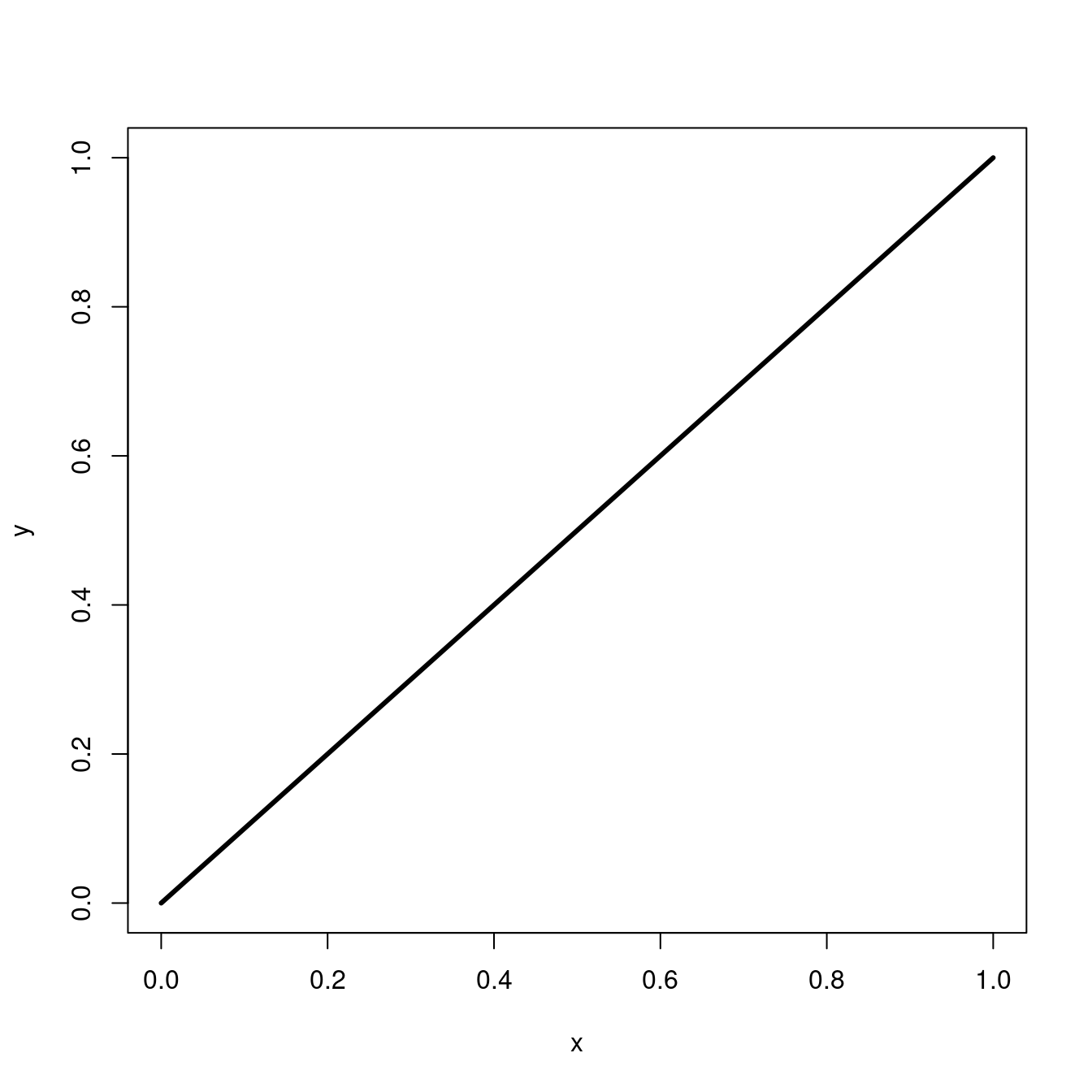
You’re probably wondering why we want to estimate this area when we already know that we can find the area of this triangle exactly using the following formula that’s very familiar to you

\[ \text{Area of triangle} = \frac{1}{2}\, \text{base} \times \text{height}. \]

The reason is that we’re using the area of a triangle as a simple example of how we can estimate quantities that we might not know an exact formula for, or that might take too long to compute exactly. So rather than computing the area of this triangle exactly, let’s try to approximate it with simulated dart throwing in R! Later, you’ll be able to apply this same technique to approximate the value of $\pi$.

Idea behind dart throwing strategy

The basic idea behind our dart throwing strategy is the following. Let’s assume that we’re going to throw darts randomly at this square. Let’s also assume that we’re equally likely to hit any point in this square. For example, we aren’t aiming the darts at the center of this square so our darts are not more likely to hit near the center than they are to hit near an edge.

If we continue to throw darts uniformly at random in this way, then we would expect about half the darts we throw to be above the line, and about half of them to be below it. If we throw a lot of darts in this way, then we should come close to filling up this square with darts.

Each time we throw a dart, we’ll keep track of whether it landed above or below the line. After throwing a lot of darts, we can estimate the area above the line by computing the fraction of dots that ended up above the line (since our square has area equal to $1$).

Sounds simple enough, right? Let’s try this out and see how well it works!

Facts we need

There are a few facts we’ll need to implement this strategy. Let’s briefly review them before diving into our code.

How do we describe this line? – We know that we can describe a line with $y = \text{slope} * x + \text{intercept}$. Here, the slope of the line is $1$ and the intercept is $0$. So our line is the $y=x$ line.
How do I figure out whether a dart landed above or below this line? – Points that land above the $y=x$ line are those with a y-coordinate that is larger than the x-coordinate. So we will throw a dart, look at its (x,y) coordinates, and know that it landed above the $y=x$ line if its y-coordinate is larger than its x-coordinate.
How do I compute the fraction of dots that landed above the line? – We’ll need to keep count of the number of dots that land above the line and the total number of darts we throw. Then we’ll compute the fraction of dots above the line with the following formula (since our square has area equal to $1$)

\[ \text{Area}\; \approx \frac{\# \text{darts above line}}{\# \text{darts total}}. \]

How do we model dart throwing in R?

There’s one more thing we need to know before we start. We need to know how to model dart throwing in R! To model dart throwing, we’re going to simulate something that lands on a point in a 2-D space. The result of a single dart throw will be a pair of (x,y)-coordinates indicating where the dart landed.

Where do we want to throw the darts?

Looking at the boundaries of the square above, we know that the x-coordinate of the dart can be any number between $0$ and $1$ and is equally likely to land anywhere between those two numbers. Similarly, the y-coordinate can be any number between $0$ and $1$ and is also equally likely to land anywhere between those two numbers. Therefore, both of these can be modeled using the runif function in R.

If you type ?runif into your R console in RStudio, you’ll see the documentation file for the runif function in the Help tab. The Usage section in the documentation shows you how to use this function. We see that this function takes in three inputs: n, min, and max.

The Arguments section in the documentation describes what these inputs mean. We see that n is the number of observations, or numbers, that we want to output. The min and max inputs give the minimum and maximum values that these numbers can take on, respectively. Since our coordinates range from $0$ to $1$, we will use min=0 and max=1. From the Usage section, we see that the default values for runif are min=0 and max=1 so we don’t need to tell R to input different min and max values.

You can try this by typing runif(1) and runif(10) into your R console. If we don’t specify min and max values, R will automatically use the default min=0 and max=1 values in the runif function.

runif(1) # no need to input `min` and `max` since the defaults are the same as what we want to use
#> [1] 0.08631393
runif(10)
#>  [1] 0.15639270 0.13532791 0.25657574 0.92804334 0.40569133 0.03364633
#>  [7] 0.82230580 0.27045160 0.01792143 0.43474603

In the first example, we input n=1 so the function returned one number between $0$ and $1$. In the second example, we input n=10 so it returned $10$ numbers between $0$ and $1$.

Notice that everything after # on the first line is commented out. That means that R will not read it so you can use it to make comments about your code for yourself and others.

How do we represent a single dart throw in terms of (x,y) coordinates?

The runif function returns $n$ random numbers between the min and max values according to a uniform distribution. We won’t go into the technical details about this but it means that it will return $n$ random numbers that are equally likely to be anywhere between the minimum input value min and the maximum input value max.

Since the result of a single dart throw is a point in 2-D space, we’ll need a pair of (x,y)-coordinates for each throw. So we will draw 2 random variables using runif for each dart throw. One way to do this is to specify the number of darts you want to throw with n. For example, if we set n=10, then that means that we want to throw 10 darts. For each dart, we will draw a pair of (x,y) coordinates resulting in a total of $2n=20$ numbers.

set.seed(123)
n <- 10 # number of darts to throw
xcoords <- runif(n)
ycoords <- runif(n)

The set.seed function here is for reproducibility of these experiments. You can change it to some other number (e.g. set.seed(1) or set.seed(2358293)) to get a different sequence of random numbers.

To view the results of the 10 dart throws we can type the variable names xcoords and ycoords into the R console to view the numbers stored in those variables. For easier viewing, we can also column-combine the variables using the cbind function.

# View the results of the 10 dart throws
xcoords
#>  [1] 0.2875775 0.7883051 0.4089769 0.8830174 0.9404673 0.0455565 0.5281055
#>  [8] 0.8924190 0.5514350 0.4566147
ycoords
#>  [1] 0.95683335 0.45333416 0.67757064 0.57263340 0.10292468 0.89982497
#>  [7] 0.24608773 0.04205953 0.32792072 0.95450365

# View in column-combined format
cbind(xcoords, ycoords) 
#>         xcoords    ycoords
#>  [1,] 0.2875775 0.95683335
#>  [2,] 0.7883051 0.45333416
#>  [3,] 0.4089769 0.67757064
#>  [4,] 0.8830174 0.57263340
#>  [5,] 0.9404673 0.10292468
#>  [6,] 0.0455565 0.89982497
#>  [7,] 0.5281055 0.24608773
#>  [8,] 0.8924190 0.04205953
#>  [9,] 0.5514350 0.32792072
#> [10,] 0.4566147 0.95450365

How do we identify the points above the line?

To identify the points above the line, we’ll use the which function in R via the following.

above <- which(ycoords > xcoords)
above
#> [1]  1  3  6 10

We can plot these points to see this visually with the following code snippet.

# Make initial plot with square boundaries and diagonal line
x <- seq(0,1,length.out = 1000)
y <- x
plot(x, y, type='l', lwd=3)

# Plot the points we simulated and color them by whether they are above or below the line
points(xcoords[above], ycoords[above], col='blue', pch=20) # Only plot points above line
points(xcoords[-above], ycoords[-above], col='orange', pch=20) # Only plot points below line

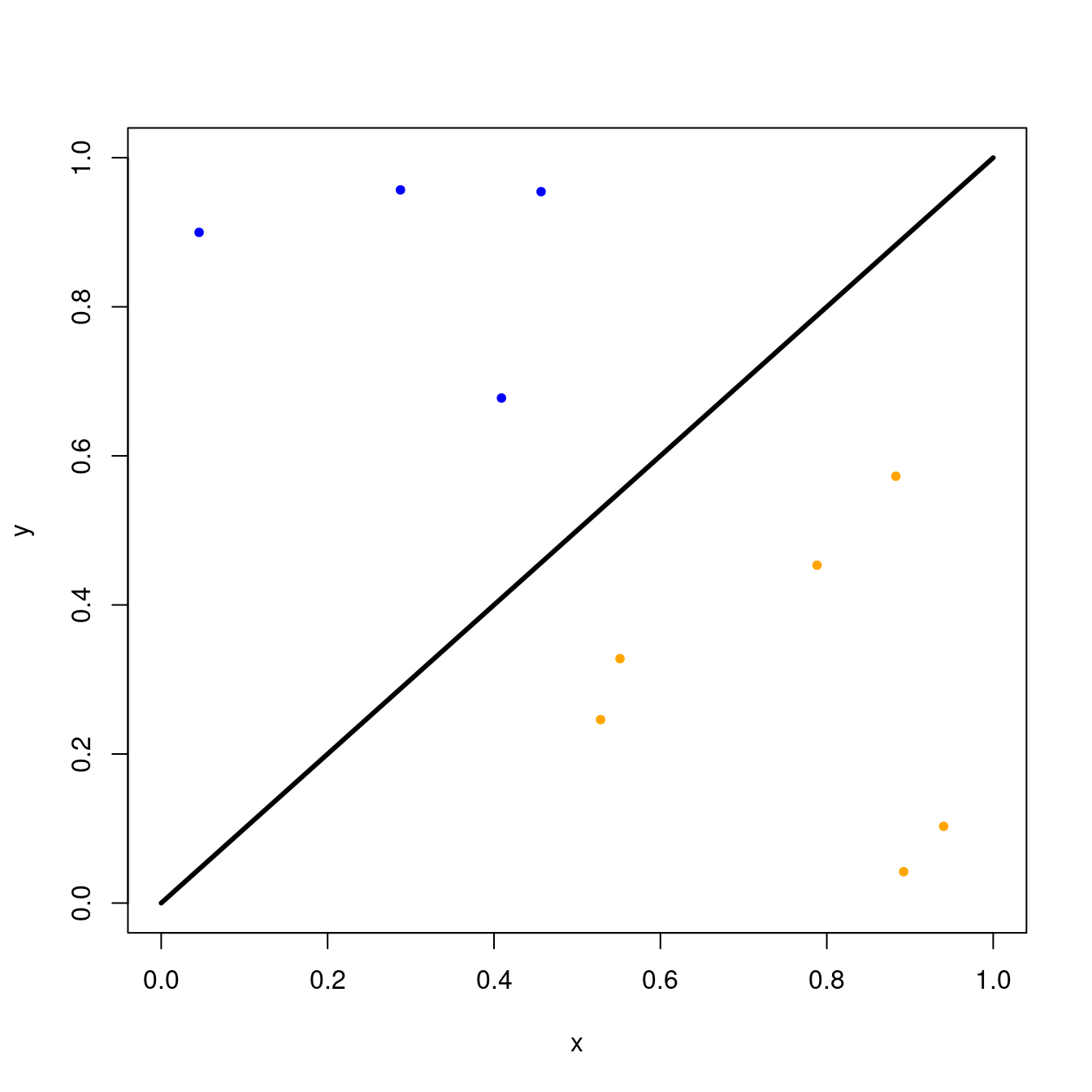
The number of darts above the line can be found by the length of the above vector.

length(above)
#> [1] 4

The current estimated area is given by the number of darts above the line divided by the total of darts thrown (since the square has area equal to $1$). Since we’ve only thrown $10$ darts, this is probably not a very good estimate yet. We’ll need to throw a lot more darts to get a better estimate.

length(above)/n
#> [1] 0.4

If we increase our number of darts to $100$, we’ll get a better estimate.

plot(x, y, type='l', lwd=3)
set.seed(1)
n <- 100
xcoords <- runif(n)
ycoords <- runif(n)
above <- which(ycoords > xcoords)
points(xcoords[above], ycoords[above], col='blue', pch=20)
points(xcoords[-above], ycoords[-above], col='orange', pch=20)

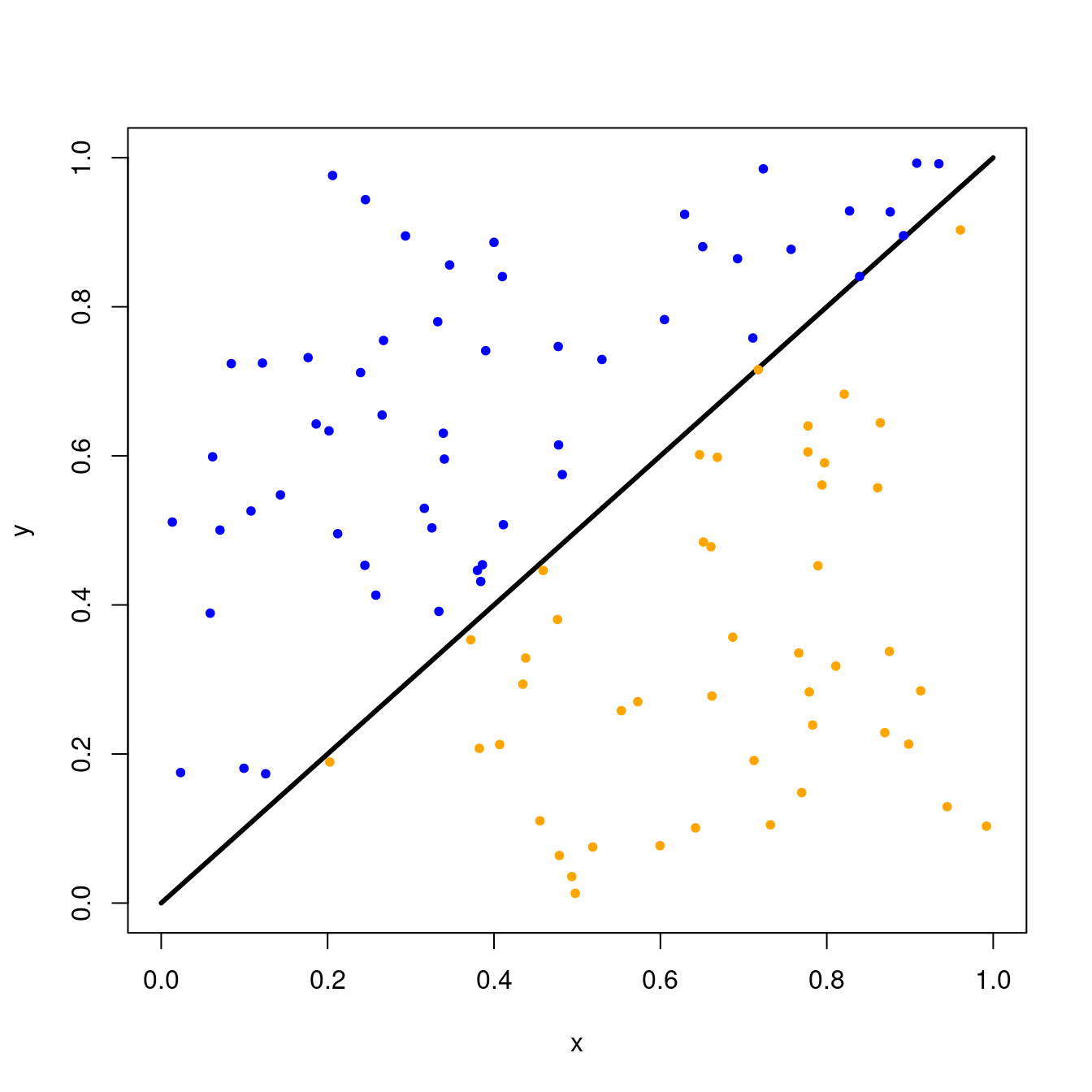
After throwing 100 darts, the estimated area of the triangle above the line is the following.

length(above)/n
#> [1] 0.54

Let’s write this all in a single function to throw $n$ darts this square and visualize the output.

Make a coding plan

Here are the things we might want to code in our function.

Draw a unit square with the $y=x$ line on the diagonal.
Simulate $n$ dart throws from the uniform distribution using the runif function.
Figure out which throws resulted in darts above the line.
Plot the output and color darts above and below the line in different colors.
Return the estimated area of the triangle above the line.

Now we’re ready to get coding!

Putting it all together in a dart-throwing function

Let’s call this function approximate_triangle. It will require an input n to tell it how many darts to throw. We’ll add another input seed so we can reproduce the random dart throws.

Your function might look something like the following. Here, I’ve added comments (after #) to explain each section in the function. Recall that these notes are for us only since R will not read anything following a #.

approximate_triangle <- function(n, seed=123) {
  # Plot square and diagonal line
  x <- seq(0,1,length.out = 1000)
  y <- x
  plot(x, y, type='l', lwd=3)
  
  # Simulate n dart throws
  set.seed(seed)
  xcoords <- runif(n)
  ycoords <- runif(n)
  
  # Determine which darts are above the line
  above <- which(ycoords > xcoords)
  
  # Plot the dart throws by color
  points(xcoords[above], ycoords[above], col='blue', pch=20)
  points(xcoords[-above], ycoords[-above], col='orange', pch=20)  
  
  # Return estimated area
  triangle <- length(above)/n
  return(triangle)
}

Now let’s try out our function with $n=5000$ dart throws!

approximate_triangle(5000)

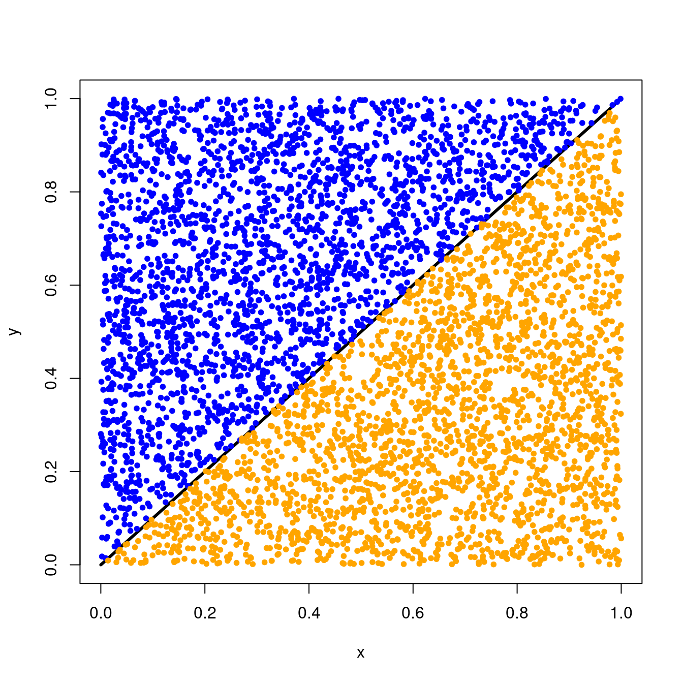
#> [1] 0.4998

So we see that with $n=5000$ dart throws, we’re getting closer to the $0.5$ area that we expect!

Approximating $\pi$

That was a bit of work to get to this point but now you’re ready to write a function to estimate pi with dart throwing in R! Recall that the area of a circle is given by

$$ \text{Area of circle} = \pi r^{2}, $$

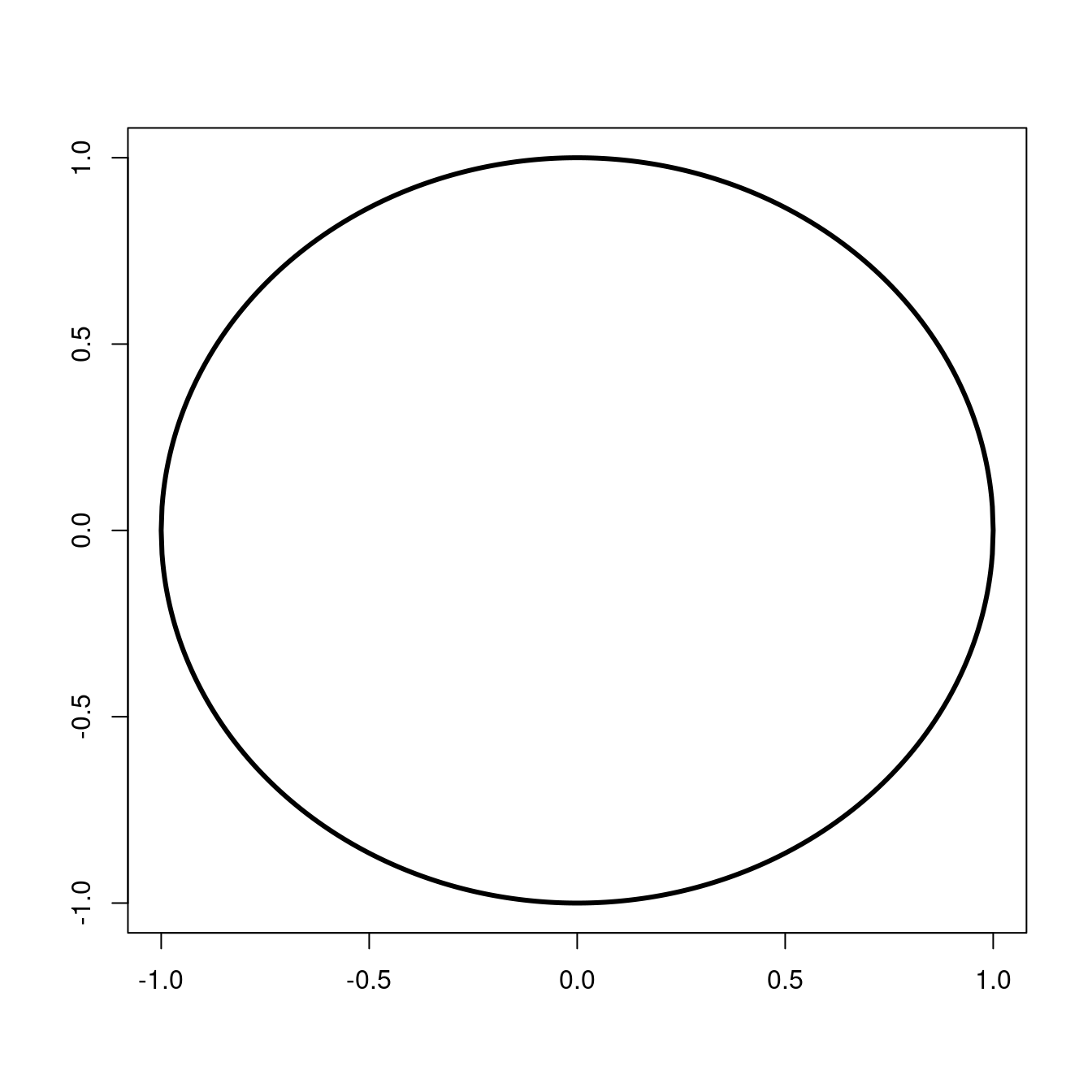
where $r$ is the radius of the circle. So a circle with radius $1$ has area equal to $\pi$. Using the same approach we employed to estimate the area of a triangle inside a square, we’ll estimate $\pi$ by estimating the area of a circle with radius $1$ inscribed inside a square. To make things simpler, let’s center the square and the circle on the origin at $(0,0)$.

Try this on your own first!

Before scrolling down for details, take some time to try this on your own! How do you think you’d do this in R? Here are some things you might want to consider.

How do we describe this circle?
Where do we want to throw the darts (in terms of (x,y)-coordinates)?
How do we know if the darts land in the circle?
How do we approximate $\pi$ using darts thrown in the circle?

Here’s some code below to get you started! Can you fill it out with what might go inside the function?

approximate_pi <- function(n=500) {
  
  # Throw darts
  xcoords <- (FILL THIS IN)
  ycoords <- (FILL THIS IN)
  
  # Identify darts in circle
  in_circle <- (FILL THIS IN)
  
  # Estimate pi
  pi <- (FILL THIS IN)
  
  return(pi)
}

Let’s work this out together!

Now that you’ve had some time to try this on your own, let’s work this out together!

How do we describe this circle? – We know that a circle with radius $1$ centered at the origin can be represented with the equation $x^{2} + y^{2} = 1$.
Where do we want to throw the darts (in terms of (x,y)-coordinates)? – Again, we will use the runif function to draw random numbers from a uniform distribution. However, since our square will be centered at the origin this time and our circle has radius $1$, we will not want to use min=0 and max=1 again. Instead, we will use runif(n, min=-1, max=1).
How do we know if the darts land in the circle? – We know that darts that land inside this circle have (x,y)-coordinates satisfying $x^{2} + y^{2} < 1$ so we will use the which function again to find these darts.
How do we approximate $\pi$ using darts thrown in the circle? – This time, our square does not have area equal to $1$. So we need to do a little scaling. We can use what we know about the areas of the circle and square to write the following

\[ \frac{\text{Area of circle}}{\text{Area of square}} = \frac{\pi r^2}{\text{base x height}} = \frac{\pi \times 1}{2 \times 2}. \]

After solving for $\pi$, we have the following

\[ \pi = 4 \times \frac{\text{Area of circle}}{\text{Area of square}}. \]

Therefore, the formula we will use to estimate $\pi$ is

\[ \pi \approx 4 \times \frac{\text{# darts in circle}}{\text{# darts total}}. \]

Okay, let’s review our code together. How does your code compare to what we have below?

approximate_pi <- function(n, seed=123) {
  
  # Plot square and circle
  x <- seq(-1, 1, length.out = 1000)
  y <- sqrt(1 - x^2)
  plot(c(x,-x), c(y,-y), type='l', lwd=3, xlab="", ylab="")
  
  # Simulate n dart throws
  set.seed(seed)
  xcoords <- runif(n, min=-1, max=1)
  ycoords <- runif(n, min=-1, max=1)
  
  # Determine which darts are inside the circle
  in_circle <- which(xcoords^2 + ycoords^2 < 1)
  
  # Plot the dart throws by color
  points(xcoords[in_circle], ycoords[in_circle], col='blue', pch=20)
  points(xcoords[-in_circle], ycoords[-in_circle], col='orange', pch=20)  
  
  # Return estimated value for pi
  pi <- 4 * (length(in_circle)/n)
  return(pi)
}

Let’s test out our code on some different values of $n$! First, let’s start with something small like $n=100$ darts.

approximate_pi(n=100, seed=123)

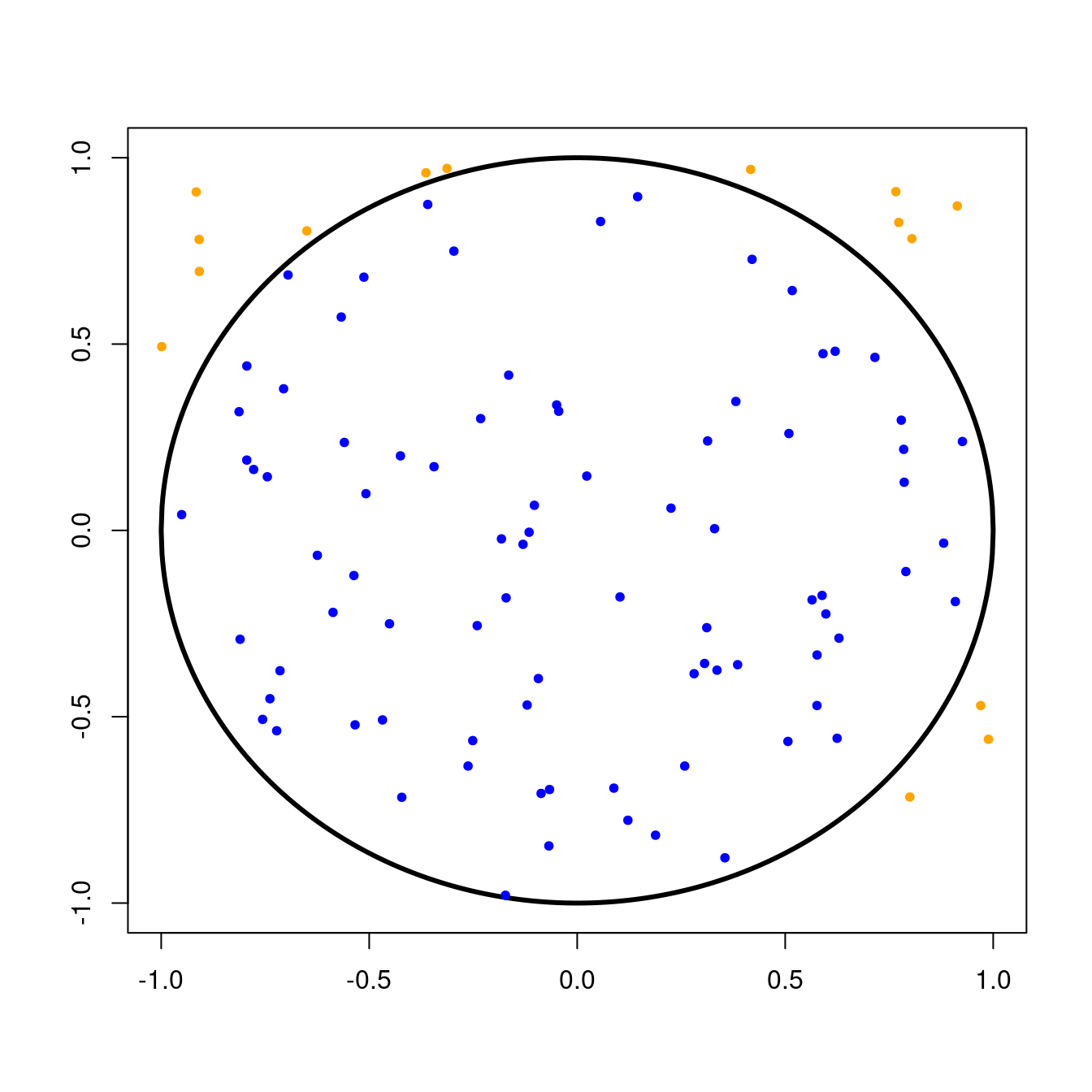
#> [1] 3.4

That’s not very accurate but we’ve only thrown $100$ darts! Let’s try throwing more darts… maybe something like $n=1000$ darts.

approximate_pi(n=1000, seed=567)

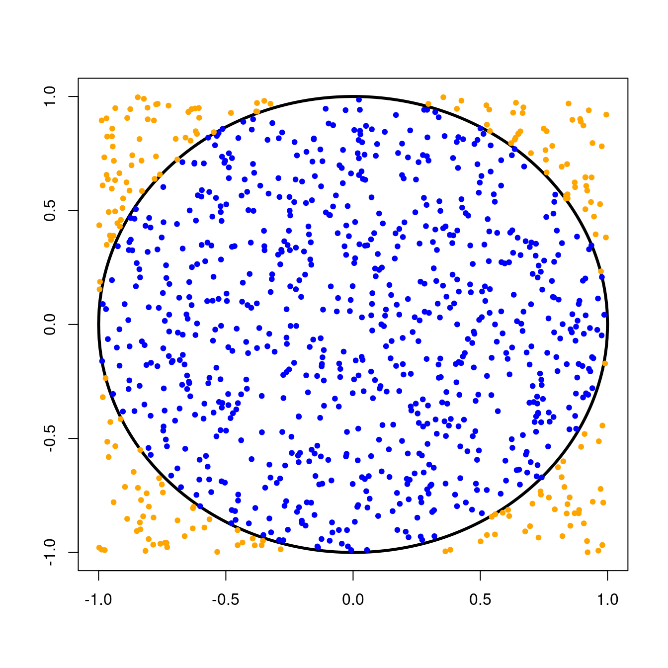
#> [1] 3.14

That’s getting better! How about (n=10000) darts?

approximate_pi(n=10000, seed=12345)

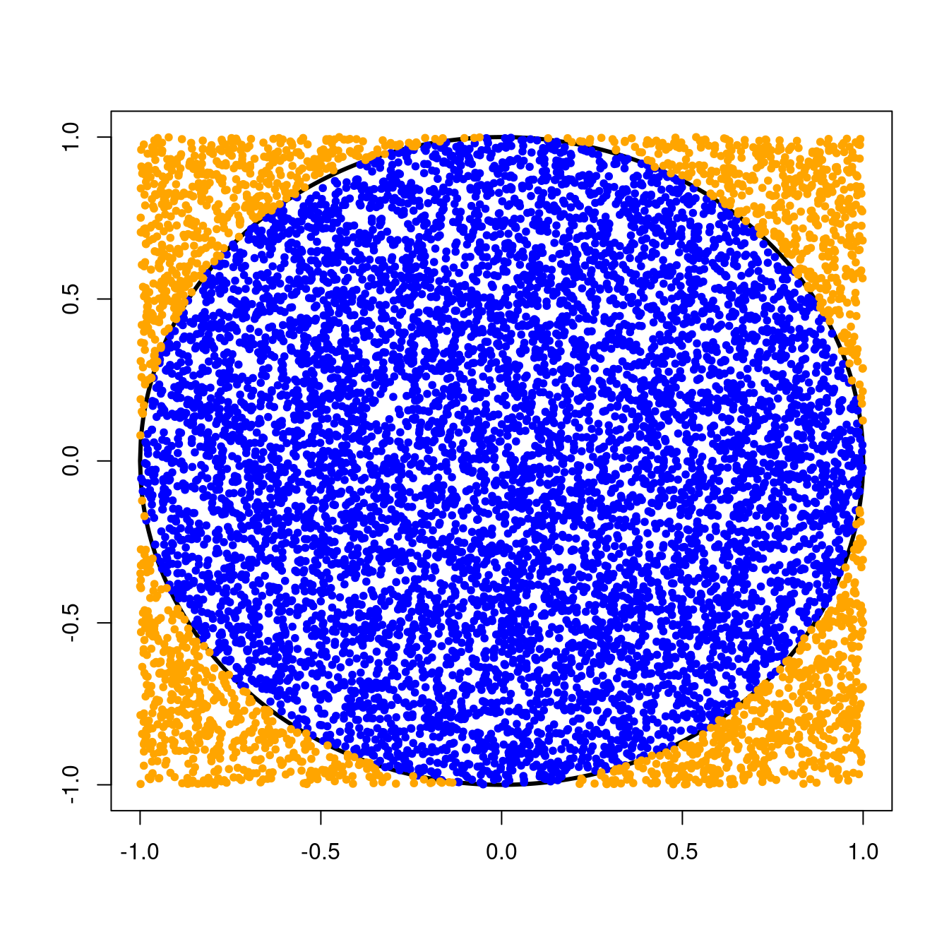
#> [1] 3.1416

Great job!

In this post, we saw how we can estimate pi with dart throwing in R! This first Code Lab illustrates how we can use algorithms to approximate quantities that might be hard to compute exactly. This is a particularly useful approach if the applications we have in mind don’t need these estimates to be extremely accurate.

We also learned some new things in R and reviewed some things from previous posts. These include creating variables using <- assignment, simulating random variables from the uniform distribution using the runif function, basic plotting using the plot function, using which to identify entries satisfying a criteria, and writing basic functions in R. Great work!