
Simple Guide to Technical Writing with LaTeX in Overleaf
You probably have your favorite software and tools for writing reports and other text documents but what can we use when we want to write things that involve math equations and symbols? Today’s post is a simple guide to getting started with technical writing with LaTeX. LaTeX is a software system that’s designed for writing that involves a lot of mathematical equations and symbols.
While it’s often accessed via various desktop clients, it’s also available for free and without additional setup requirements on Overleaf. Overleaf is an online LaTeX editor that’s particularly great for collaborations!
Getting started with Overleaf
To start using Overleaf, we’ll need to sign up for a free account at https://www.overleaf.com/. Although we can register and log in with several existing accounts, including your Google account, we can also create an account with just an email address.

Once we’ve created an account, we can start making a new project!

We’ll use the example template on Overleaf as a starting point for us. To start using this template, we can select it from the drop down menu below.
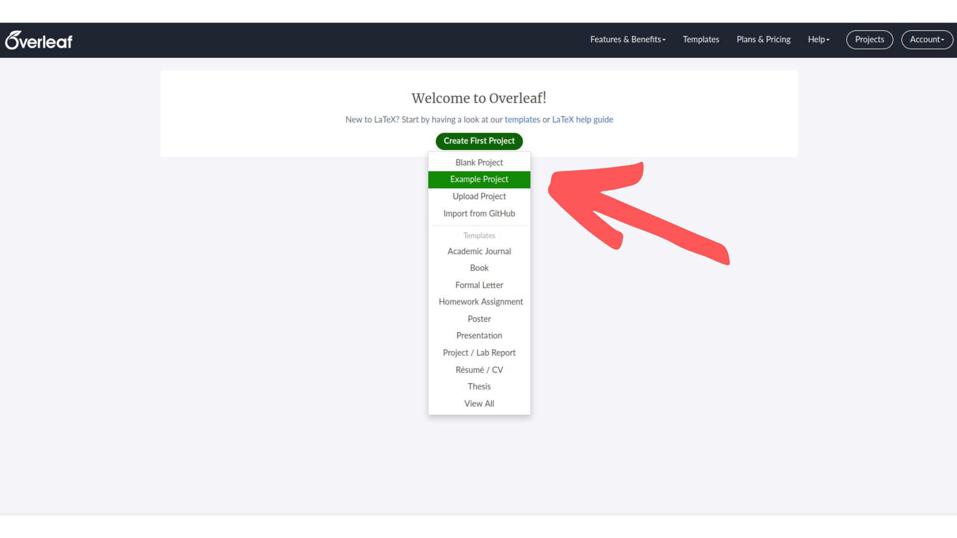
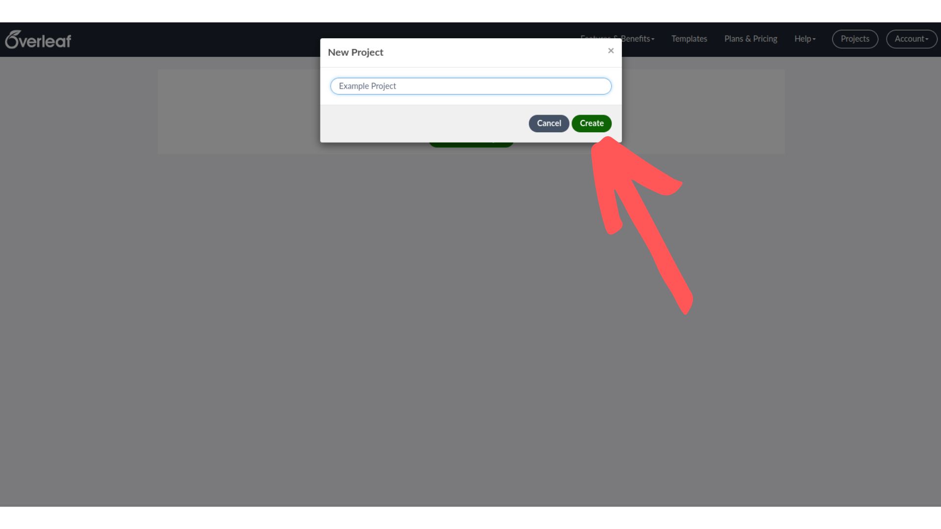
If we want to rename the project, we can set a new project name in the prompt below. We can also change the project name later so no pressure coming up with a particularly good name for the project right now!
Working on projects in Overleaf
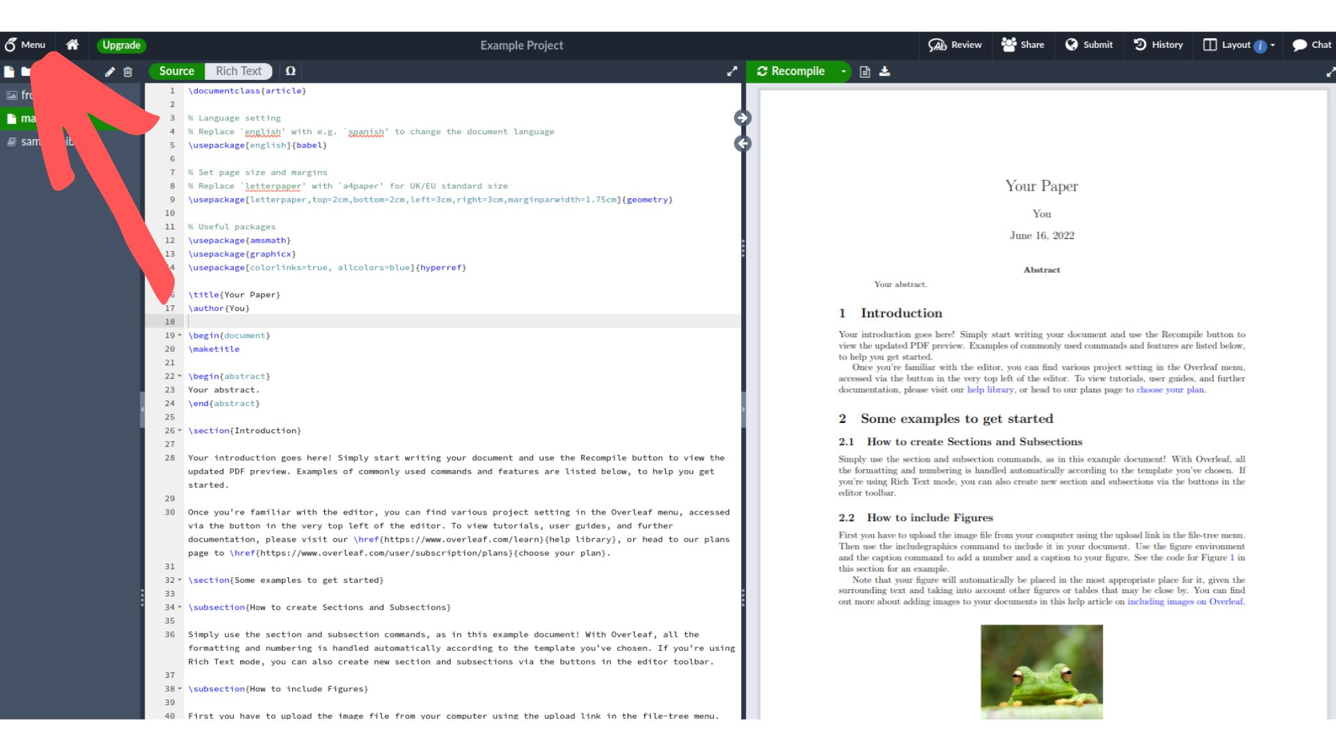
The image below shows what a project looks like in Overleaf. One of the first things to notice is that we can change the editor font size from the Menu option in the top left-hand corner.
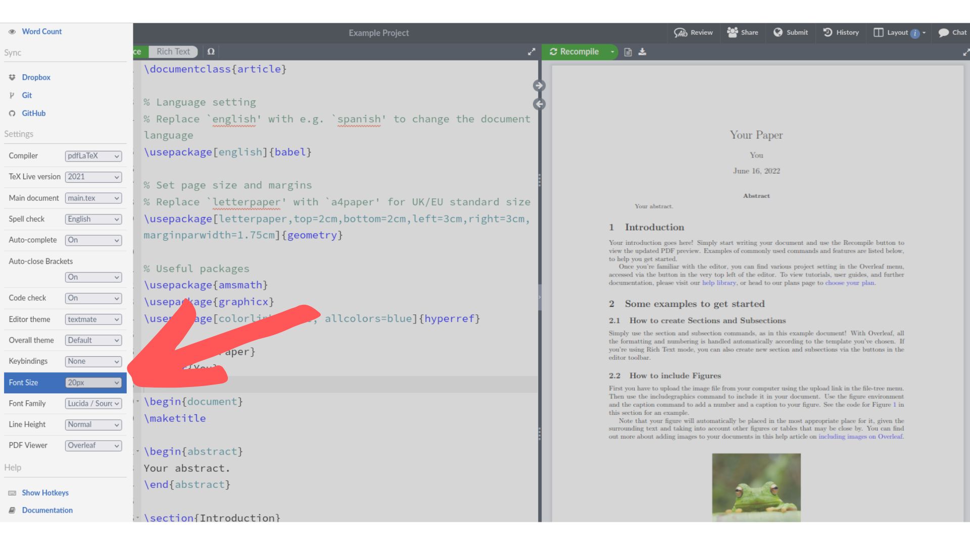
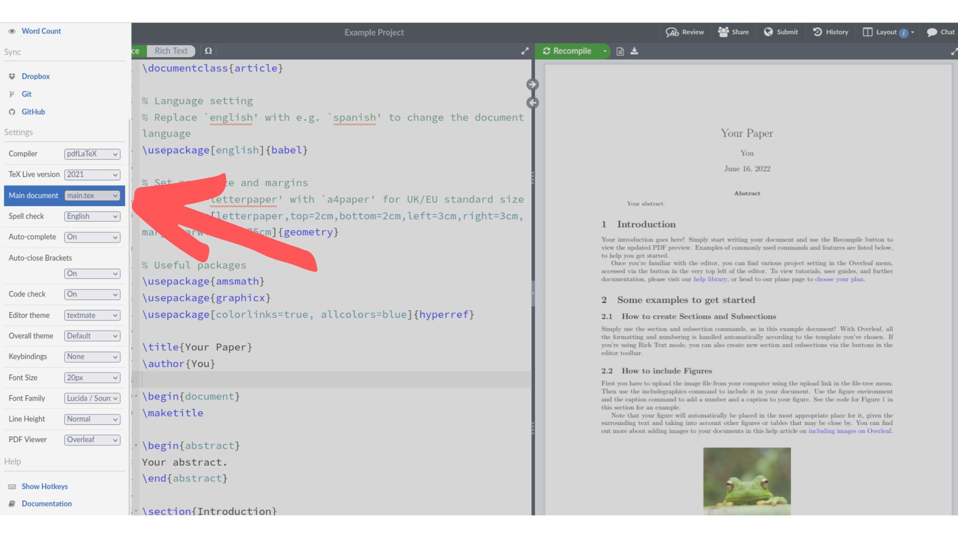
To change the editor font size, we first select Menu (see the arrow above), and then input the font size we want in the Font Size option below (see the arrow below). In the image below, I’ve selected 20px so that we can read the text on this screen together.
Another useful item that we can access from Menu is the Main Document input (see the arrow below). The file listed in this area is the one that is automatically compiled in the project. Typically, this is the main.tex file but it can be any file that ends with .tex. Sometimes, we might have multiple .tex files. In that case, we can select the primary .tex document from this input.
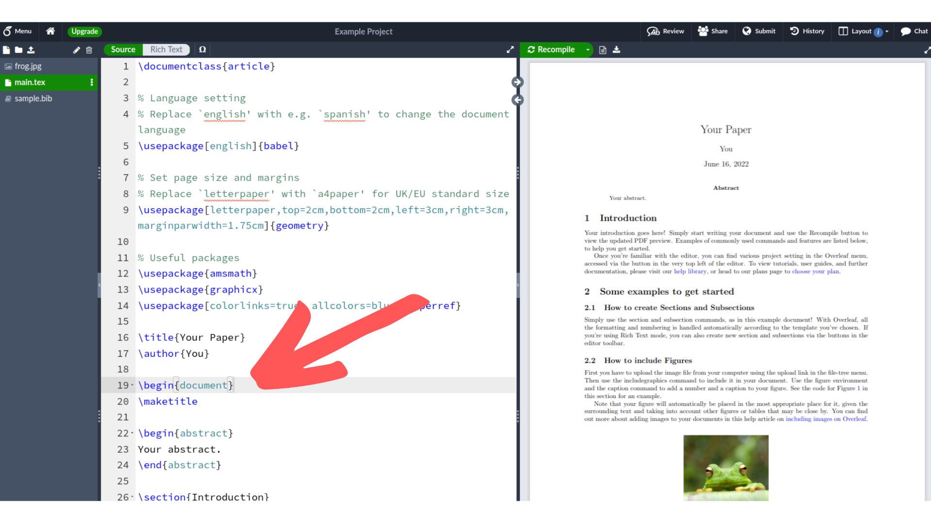
Now let’s exit the Menu and go back to our project. We’ve selected main.tex from the far left panel so the editor window on the left side shows us what we have inside main.tex. Meanwhile, the right side panel automatically compiles main.tex and shows us a preview of main.pdf.
The part that we see in the output on the right starts at begin{docment} below (see the arrow below).
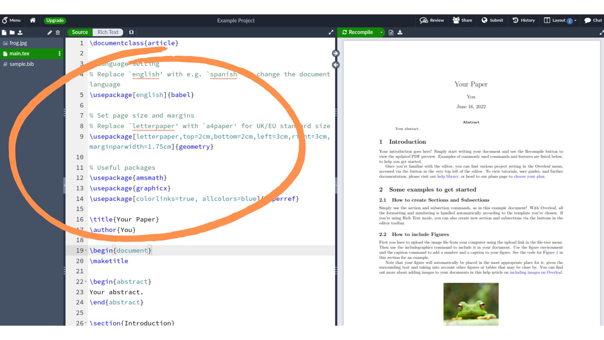
The portion above begin{document} contains our document header (see the part circled in orange below). In this header area, we can input different packages we want to use with the \usepackage{} command. This example template already includes some commonly used packages for typesetting math so we can get started with the ones already here!
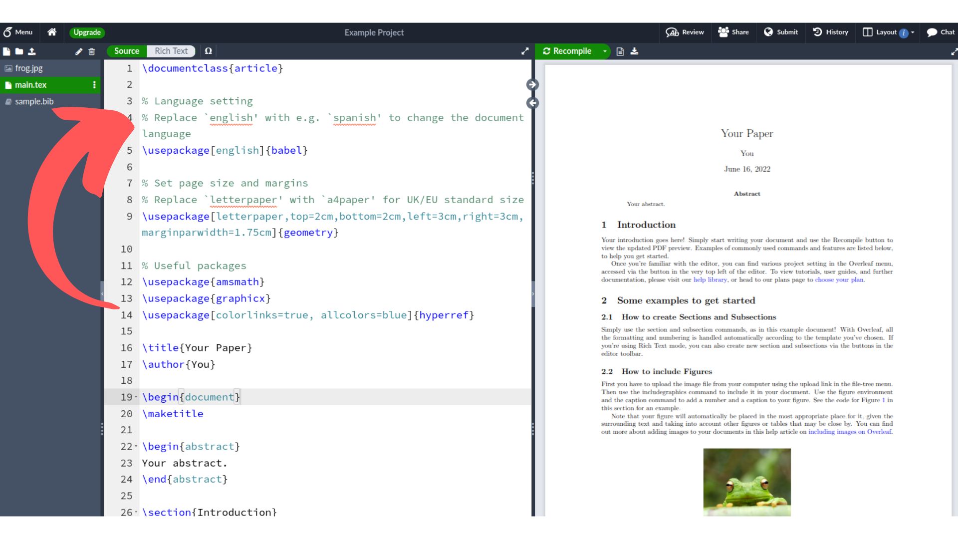
In the image below, we can see some text in green (see the arrow below) that starts with %. The % indicates a comment. A comment is text that we can leave for ourselves and other users of our code. Anything following the % will not be read by the LaTeX compiler so we can leave notes to ourselves about why we’re calling certain packages, or what a certain chunk of code does.
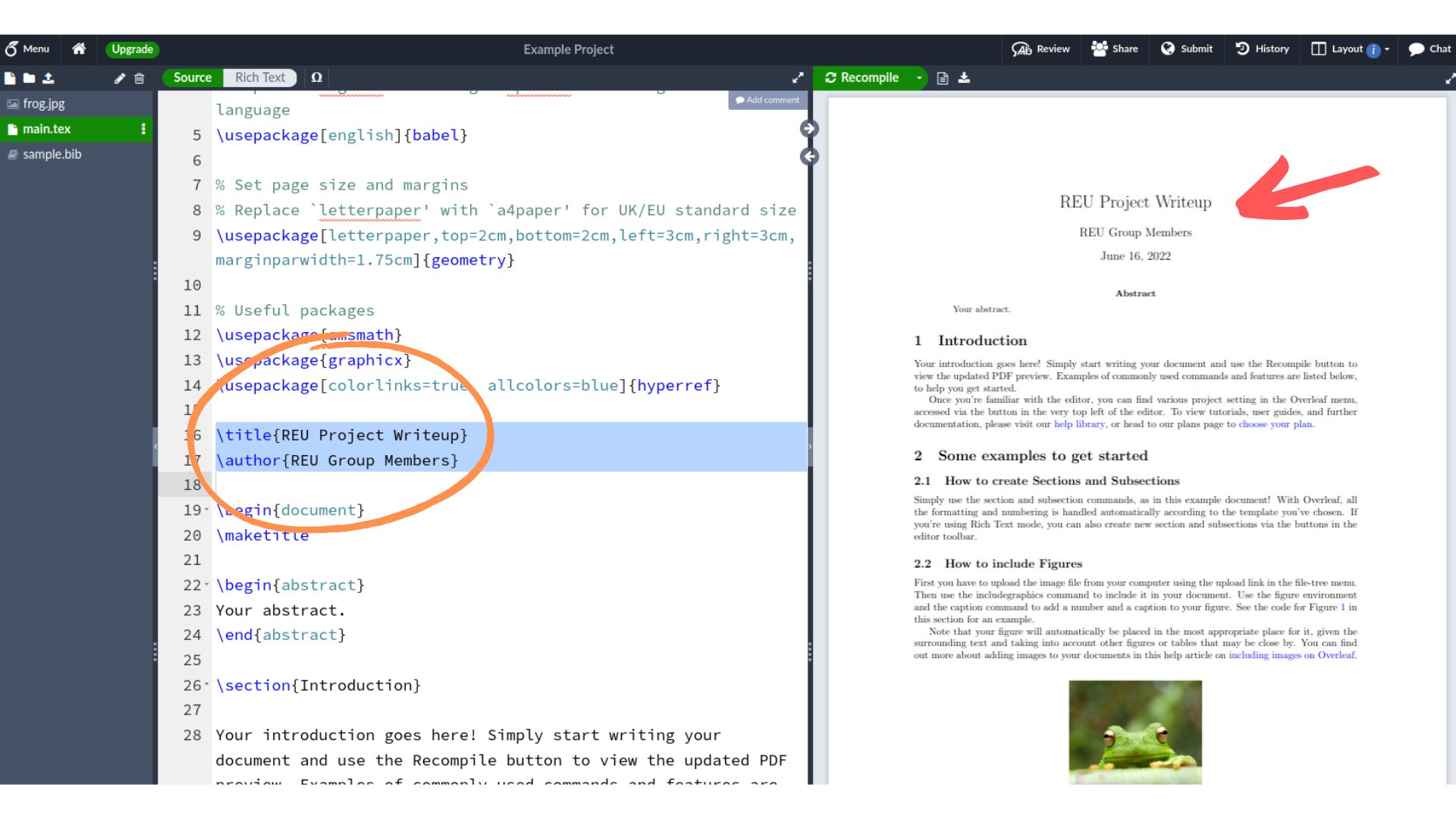
The \title{} and \author{} commands (at the orange circled text below) are where we input the title of our project and any authors we want to list. Whatever we input in these commands shows up as the title when we call the \maketitle command.
Making sections and subsections
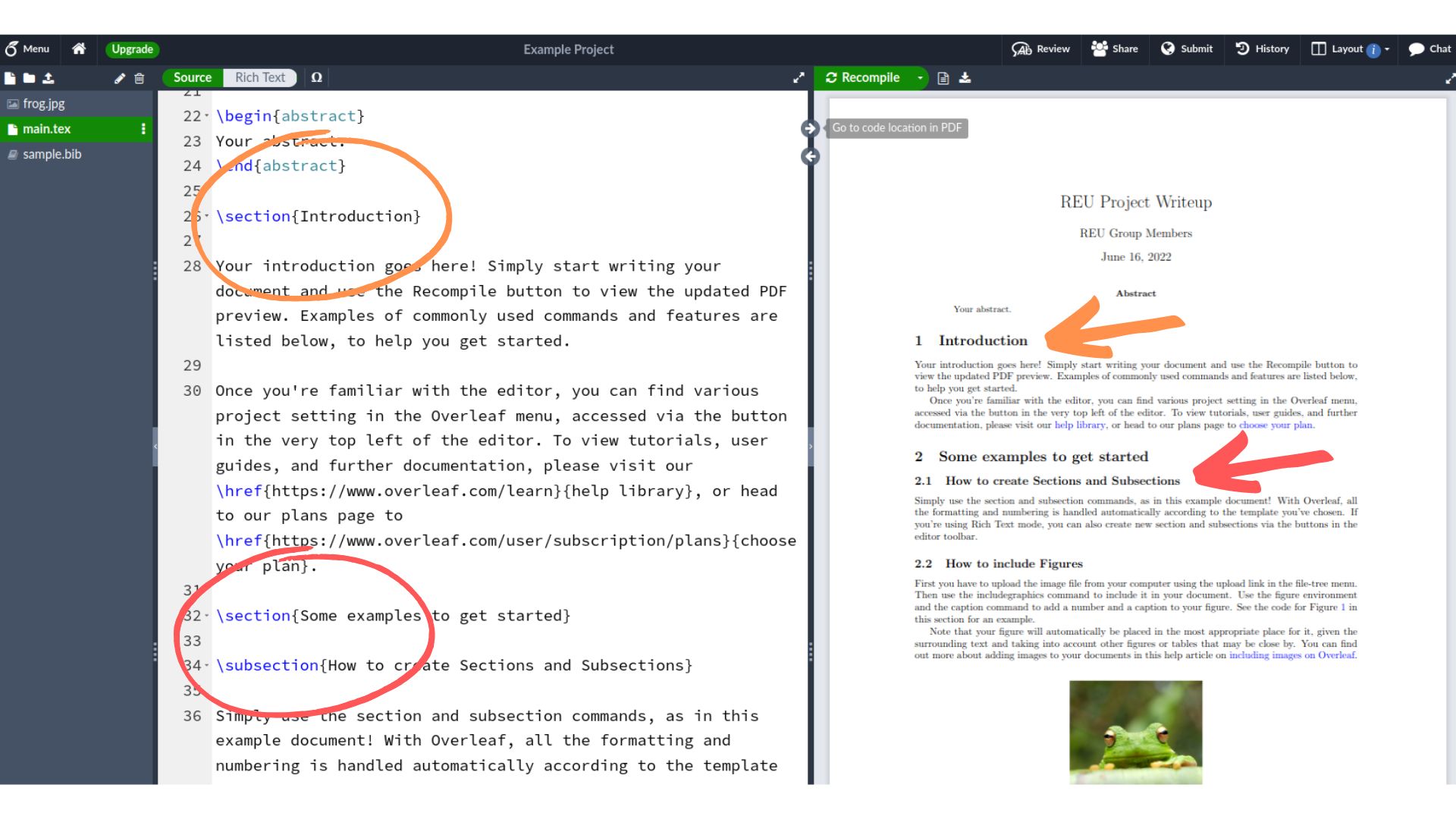
We can make new sections and subsections with the \section{} and \subsection{} commands, respectively (see the circled text below). The output on the preview panel shows that the section headings are larger and boldfaced compared with the rest of the text (see the arrows below).
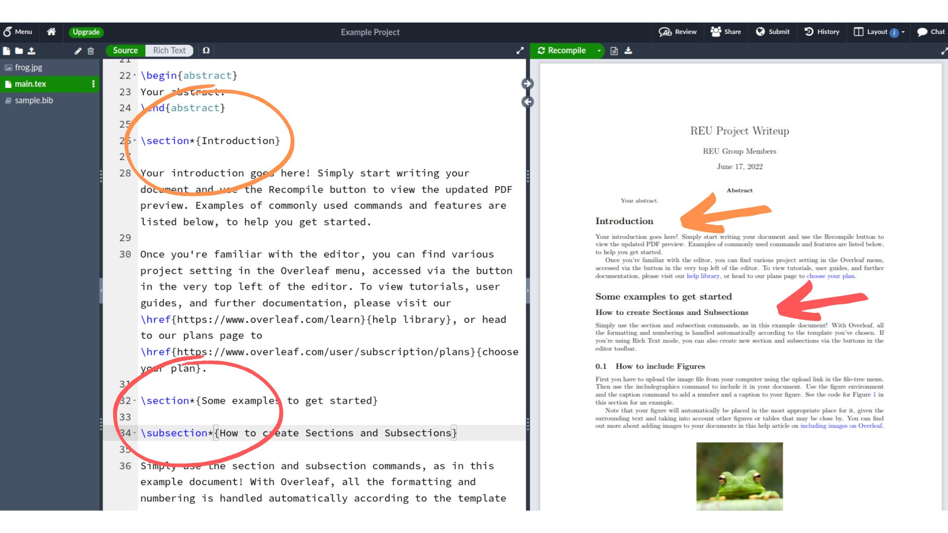
By default, the sections and subsections are numbered in the order that they appear in the document. If we want to remove the numbers, we can do that by using the commands \section*{} and \subsection*{} instead.
Adding links to online materials
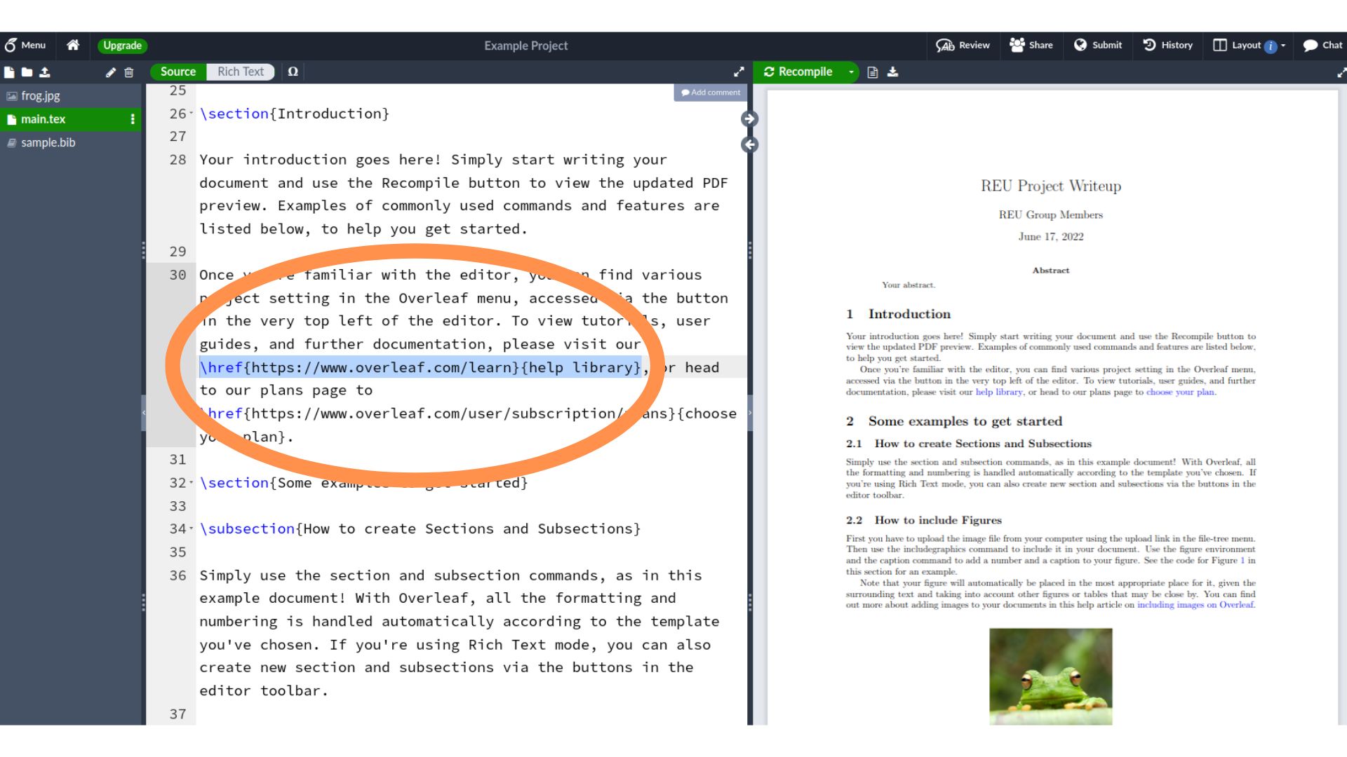
We can add links to things online with the \href{}{} command. The first input in this command is the url, or web address, of the item we want to link to. We put this first input inside the first set of curly brackets. The second input is the text that shows up as the link. We put this second input in the second set of curly brackets.
Inserting and referencing figures
To add figures in our document, we can use the \includegraphics{} command by itself, where the input is the location of the file in your project directory structure. In the image below, the input is frog.jpg because the frog.jpg file is located in the same file level as main.tex. If we store images in a subfolder called images, the input would be input/frog.jpg instead.
To specify the width of the inserted figure, we can add rectangular brackets inside the \includegrahics{} command with \includegraphics[]{}. In the image below, the width is set to 0.3 times of the text width in the document. Since \textwidth is a parameter that is already defined within LaTeX, we don’t have to define it separately before using it.
If we include the \includegraphics{} command inside the \begin{figure} ... \end{figure} commands, we can additionally add a figure caption and reference the figure in the text. These are added via the \cation{} and \label{} commands (see the text circled in orange below).
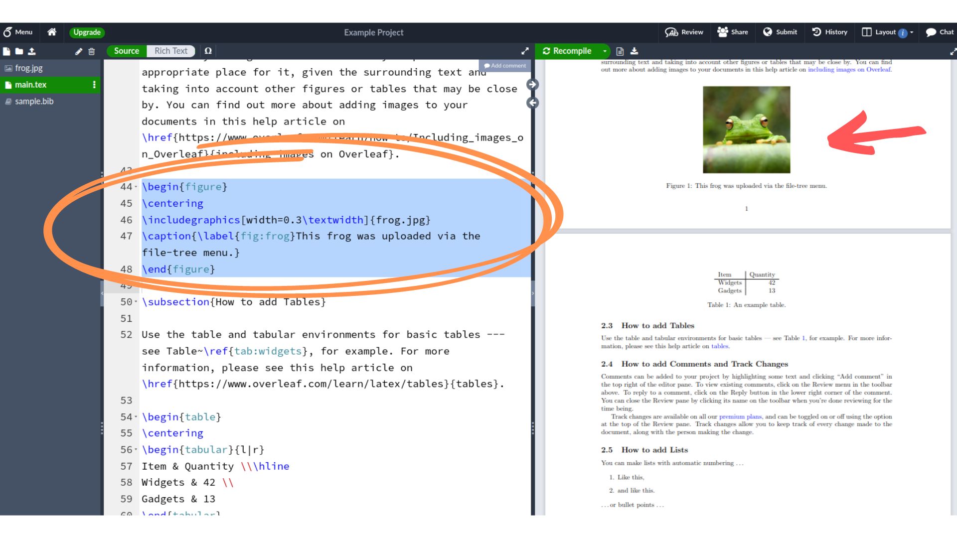
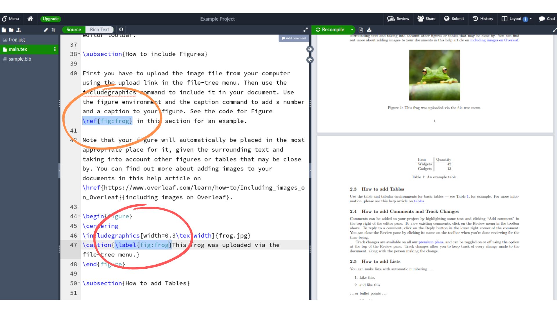
We can reference a figure within a document with the \ref{} command. The input to this command is the label of the figure we want to reference and again goes inside the curly brackets. To find this relevant label, we go to the \label{} command of the figure we want to reference and copy and paste the text inside the curly brackets into the \ref{} command.
For example, in the image below, the label for the frog figure is fig:frog, which we find from \label{fig:frog}. So we will use \ref{fig:frog} wherever we want the reference to this figure to appear in the text.
Inserting and referencing tables
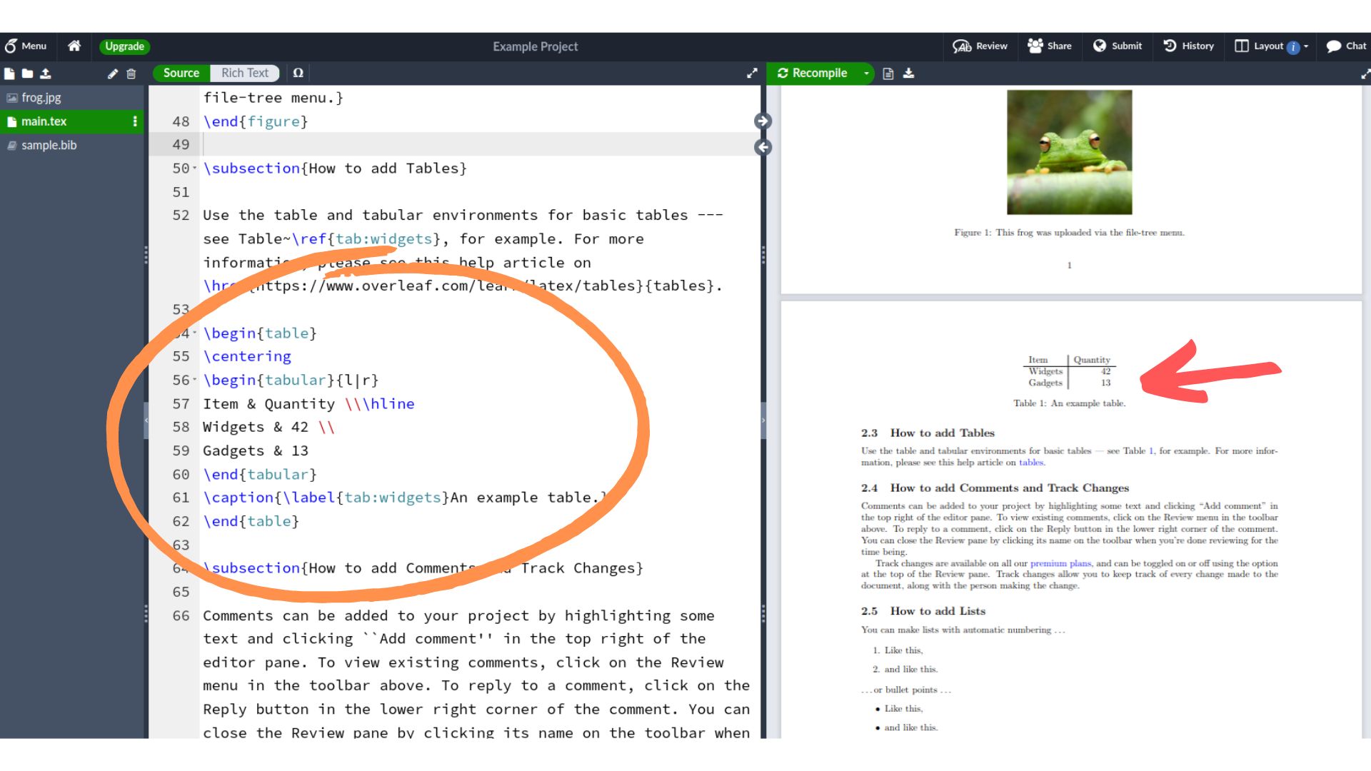
To add a table (see the red arrow below) to the document, we insert a chunk of code that begins with \begin{table} and ends of \end{table} (see text circled in orange below).
- New columns in the table are indicated by
&and new rows are indicated by\\. - The
{l|r}in line 56 below indicate that the text in the first and second columns should be aligned to the left and right, respectively. - The
\hlinein line 57 creates a horizontal line.
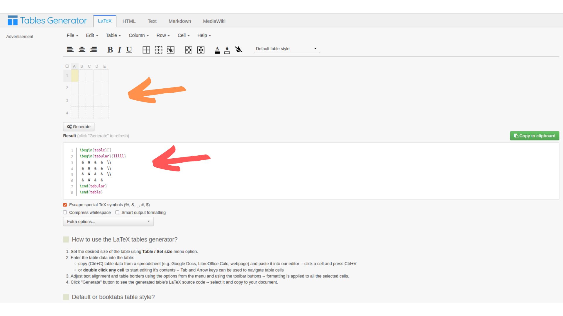
Making tables in LaTeX can be a little tricky. A very useful tool for inserting tables in LaTeX is the online table generator at https://www.tablesgenerator.com/. To use this table generator, we type the text and numbers we want in the top part of the website (see the orange arrow). The website will then automatically generate LaTeX code for our table (see the red arrow). We then copy and paste this code snippet directly into our .tex file to get the table into our document.
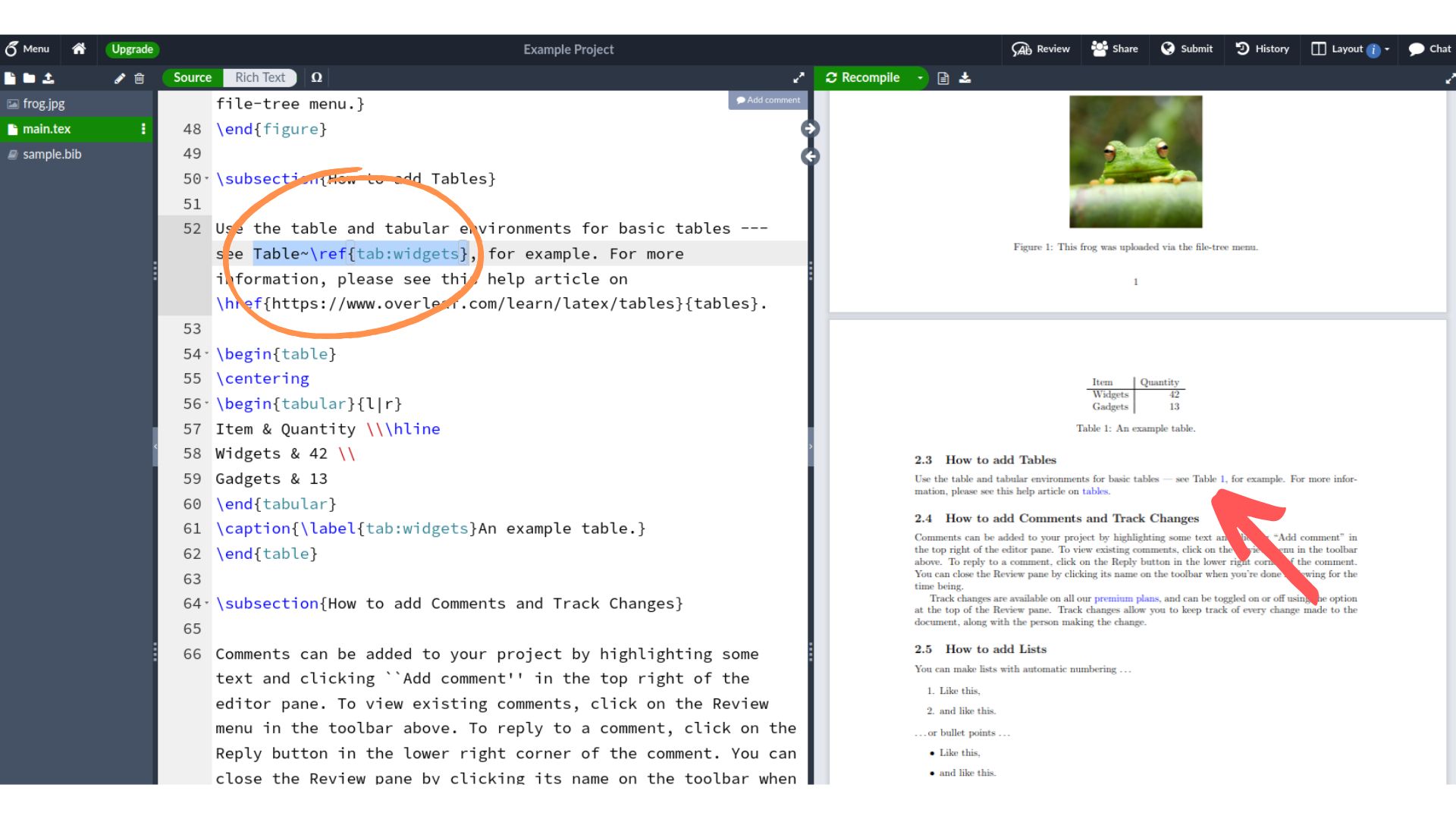
We can also reference this table in the same way that we referenced figures earlier. We simply copy and paste the label for the table into the \ref{} command wherever we want the reference to appear in the text. The red arrow below shows how the reference then appears in the text.
Inserting numbered and bulleted lists
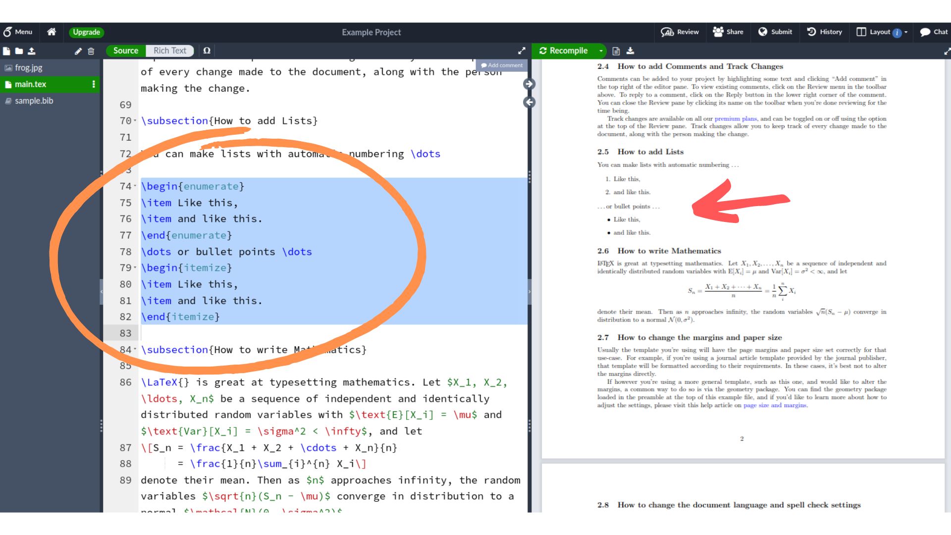
We can add numbered lists by including them within the \begin{enumerate} and \end{enumerate} commands as follows. We indicate a new item in the list by preceding it with \item. The items in the list will be numbered in the order that they are listed below.
\begin{enumerate}
  \item First item goes here
  \item Second item goes here
\end{enumerate}
We can similarly add bulleted lists by including them within the \begin{itemize} and \end{itemize} commands as follows. Again, each new item is indicated by \item and the items in the list will appear in the order that they are listed.
\begin{itemize}
  \item First item goes here
  \item Second item goes here
  \item Third item goes here
\end{itemize}
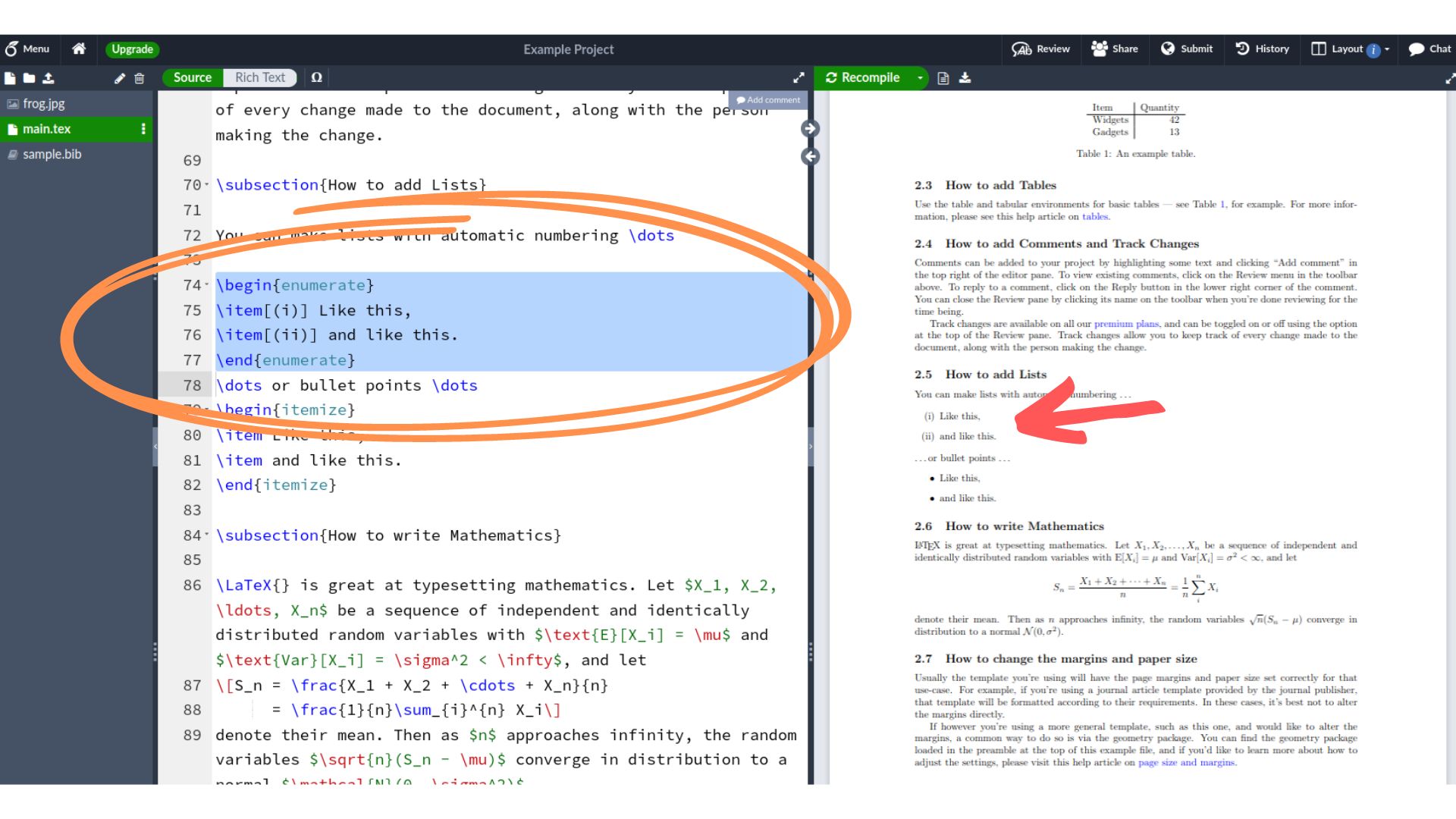
We can override the default numbers within the enumerate environment by inserting brackets after the \item command as follows. The red arrow below shows how the numbering then changes in the text.
\begin{enumerate}
  \item[(i)] First item goes here
  \item[(ii)] Second item goes here
\end{enumerate}
Inserting math
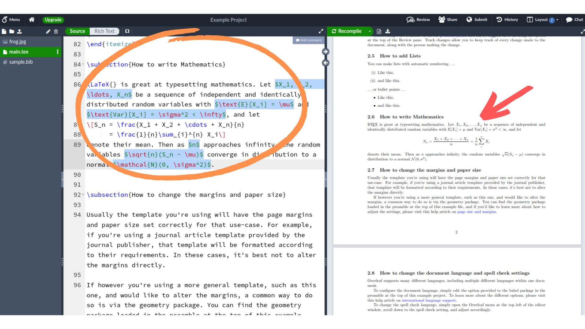
There are two ways to insert math. The first is inline as part of the text in a paragraph. The second is outside of the paragraph. To insert inline math, we simply include the math between two dollar signs. In the following example, we inserted the following text inside our document.
Let $X_{1}, X_{2}, \dots, X_{n}$ be a sequence of independent and identically distributed random variables...
This text appears as the following in the text.
Let $X_{1}, X_{2}, \ldots, X_{n}$ be a sequence of independent and identically distributed random variables…
Below are some other useful things to know about inserting mathematical formulas.
- We indicate subscripts with an underscore
_. - We indicate superscripts with a caret
^. - Text is naturally italicized within the math environment. If we want the text to appear normally, we specify it within
\text{}. - We can use
\cdotto get $\cdot$,\dotsto get $\dots$,\cdotsto get $\cdots$, and\vdotsto get $\vdots$. - We can input fractions with
\frac{}{}. For example,\frac{1}{2}appears as $\frac{1}{2}$. - We can use
\sqrt{}to indicate the square root function.
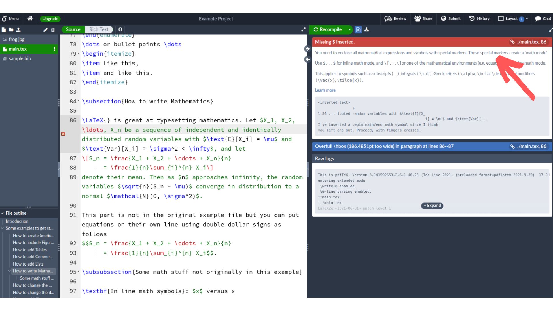
If we forget to include a closing $, we will run into compilation errors. This is very common and easily corrected by identifying the line that is missing the dollar sign from the error message and inserting it where it belongs.
Sometimes, we may want to insert stand-alone math equations. There are several ways to do this. The first is to enclose it within \[ ... \] or $$ ... $$. For example,
\[
S_n = \frac{X_{1} + X_{2} + \cdots + X_{n}}{n} = \frac{1}{n} \sum_{i=1}^{n} X_{i}
\]
appears as
\[S_n = \frac{X_{1} + X_{2} + \cdots + X_{n}}{n} = \frac{1}{n} \sum_{i=1}^{n} X_{i}.\]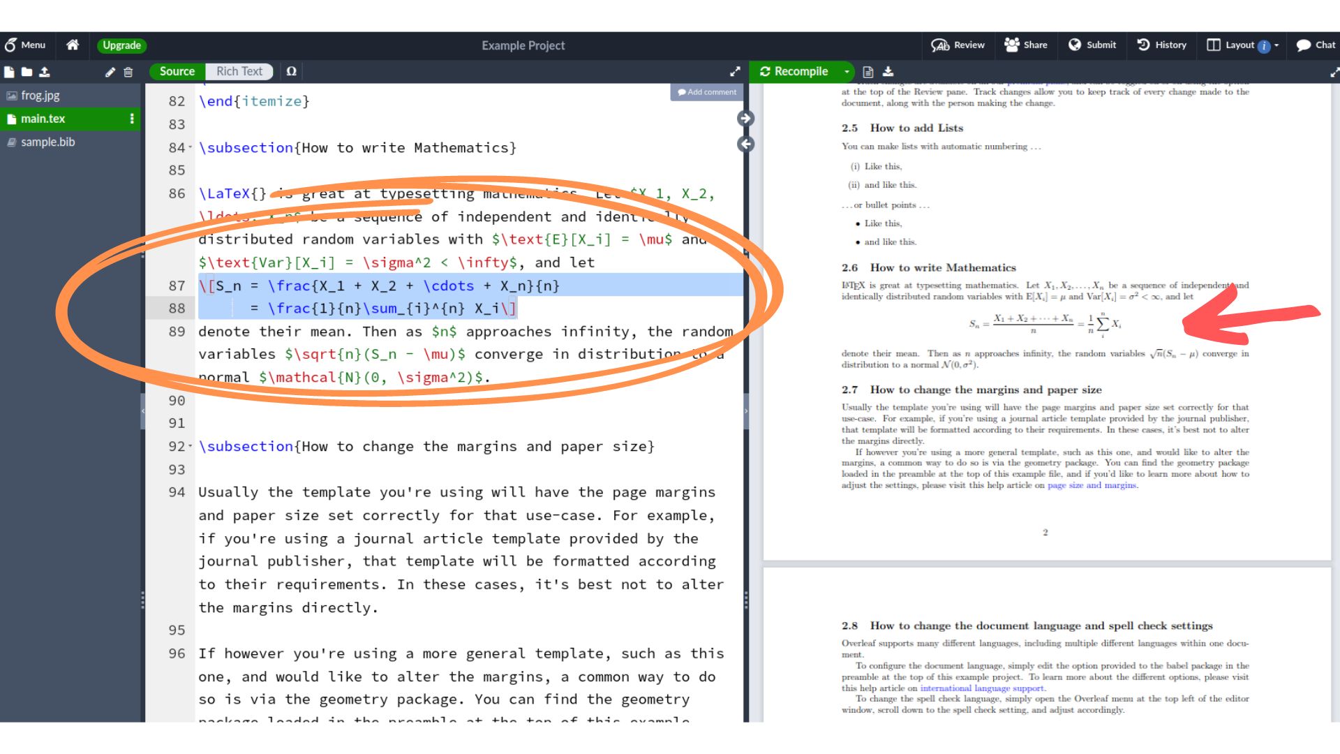
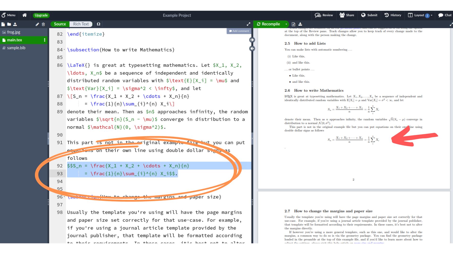
Similarly, if we replace \[ ... \] with double dollar signs,
$$
S_n = \frac{X_{1} + X_{2} + \cdots + X_{n}}{n} = \frac{1}{n} \sum_{i=1}^{n} X_{i}
$$
also appears as
\[S_n = \frac{X_{1} + X_{2} + \cdots + X_{n}}{n} = \frac{1}{n} \sum_{i=1}^{n} X_{i}.\]We can also achieve the same stand-alone math equation by inputting the math within \begin{equation} ... \end{equation} to utilize the equation environment.
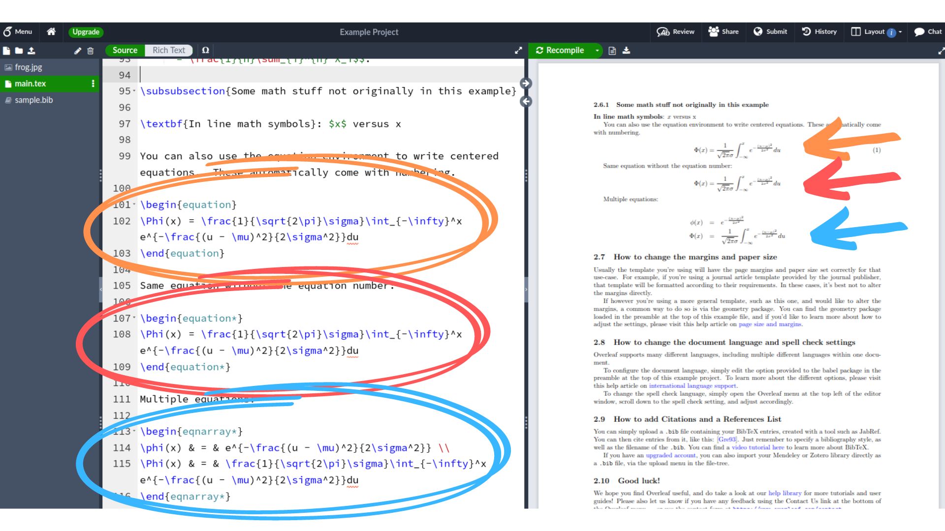
If we additionally want to align our math equations over multiple lines, we can do that within the eqnarray environment by inputting the math between \begin{eqnarray} ... \end{eqnarray}. For multiple lines, we typically align them at the equal sign = by placing & on either side of =. To indicate a new line, we again use \\.
The image below shows some examples. The colored arrows show how the output appears in the document. By default, the equation and eqnarray environments will add equation numbers. If we want to remove the numbering, we add an asterisk as in \begin{equation*} ... \end{equation*} or \begin{eqnarray*} ... \end{eqnarray*}.
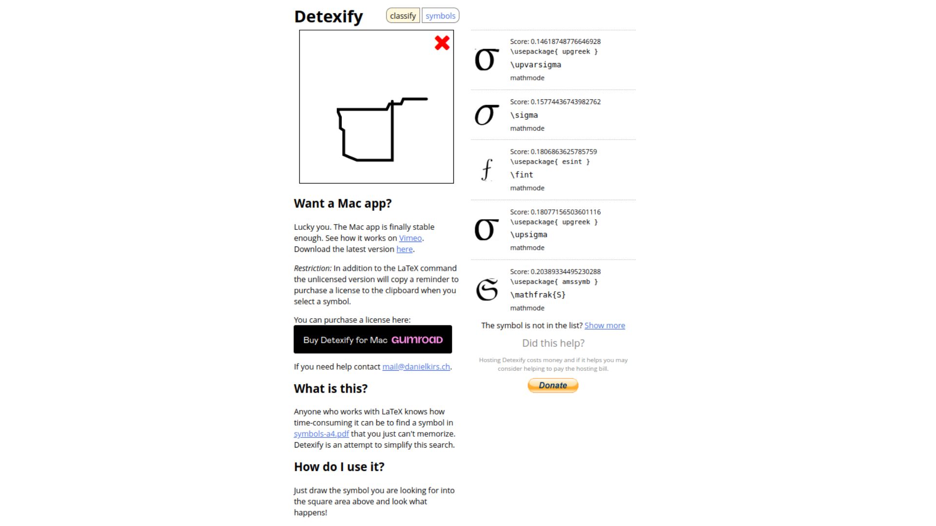
Sometimes it can be a little tricky to remember the LaTeX command for a particular math symbol. One very useful (and free) tool for this is Detexify!
To find out the LaTeX command for a particular symbol, we can draw the symbol (for example, with your mouse) in the box on the Detexify site. When we’re done, it will offer several possible matches for our drawing and show them on the right of the box!
Inserting citations and references
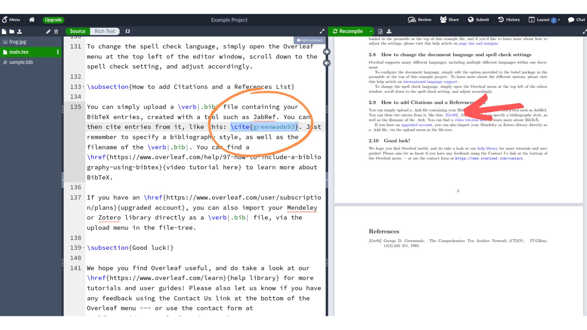
To insert a citation from something we want to include in a bibliography, we can use the \cite{} command (see the orange circled text below). Then to reference a particular item, we insert its label (or BibTeX key) inside the curly brackets in the \cite{} command just like we do when we want to reference a table or figure.
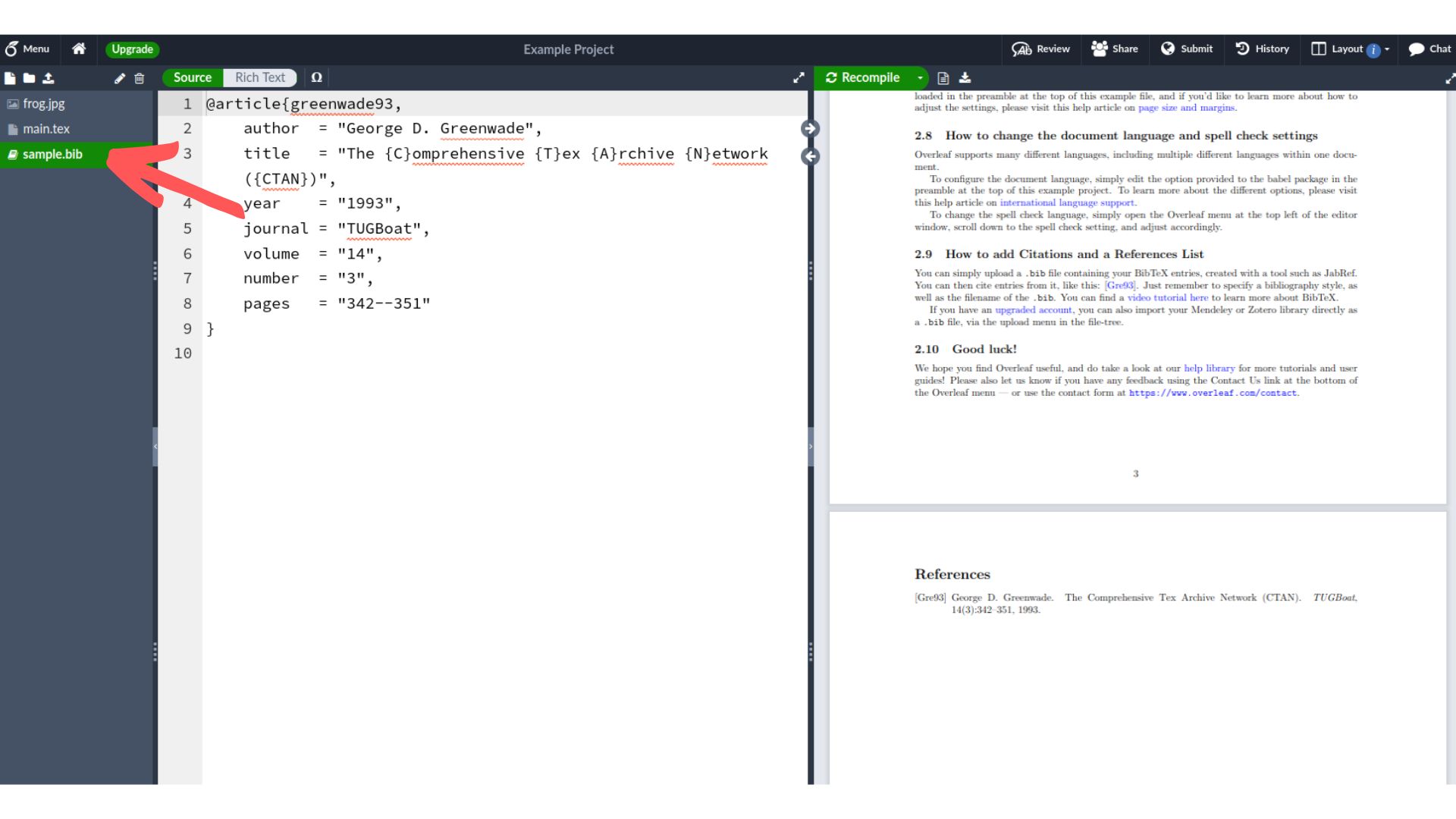
Before we cite something, we first need a label for the entry. we first add its entry inside our .bib file. In the image below, we’re looking at the contents of the sample.bib file. We can see that there is one bibliographic entry in this file. Since the entry begins with @article, we know that this entry is for a journal article.
The first input after the opening curly bracket is the reference label for this bibliographic entry. In the example below, this is greenwade93. So to cite this article, we would use the command \cite{greenwade93} wherever we want the citation to appear in the text.
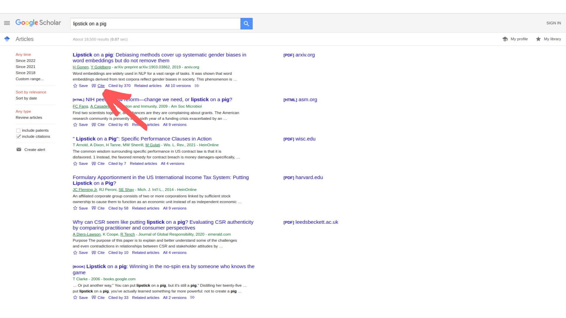
So how do we find BibTeX entries for things that we want to cite? For journal articles, a very common method for this is to search by article name and/or authors in Google Scholar.
In the example below, we’ve input the “Lipstick on a Pig” article into the search bar. In this case, it’s the first entry that shows up in the search. We then click on the Cite link (see arrow below) to get a list of options for how to cite this article.
Below is the box that pops up when we click on Cite for the article. To find the BibTeX entry for this article, we click on the BibTeX link at the bottom of the box (see arrow below).
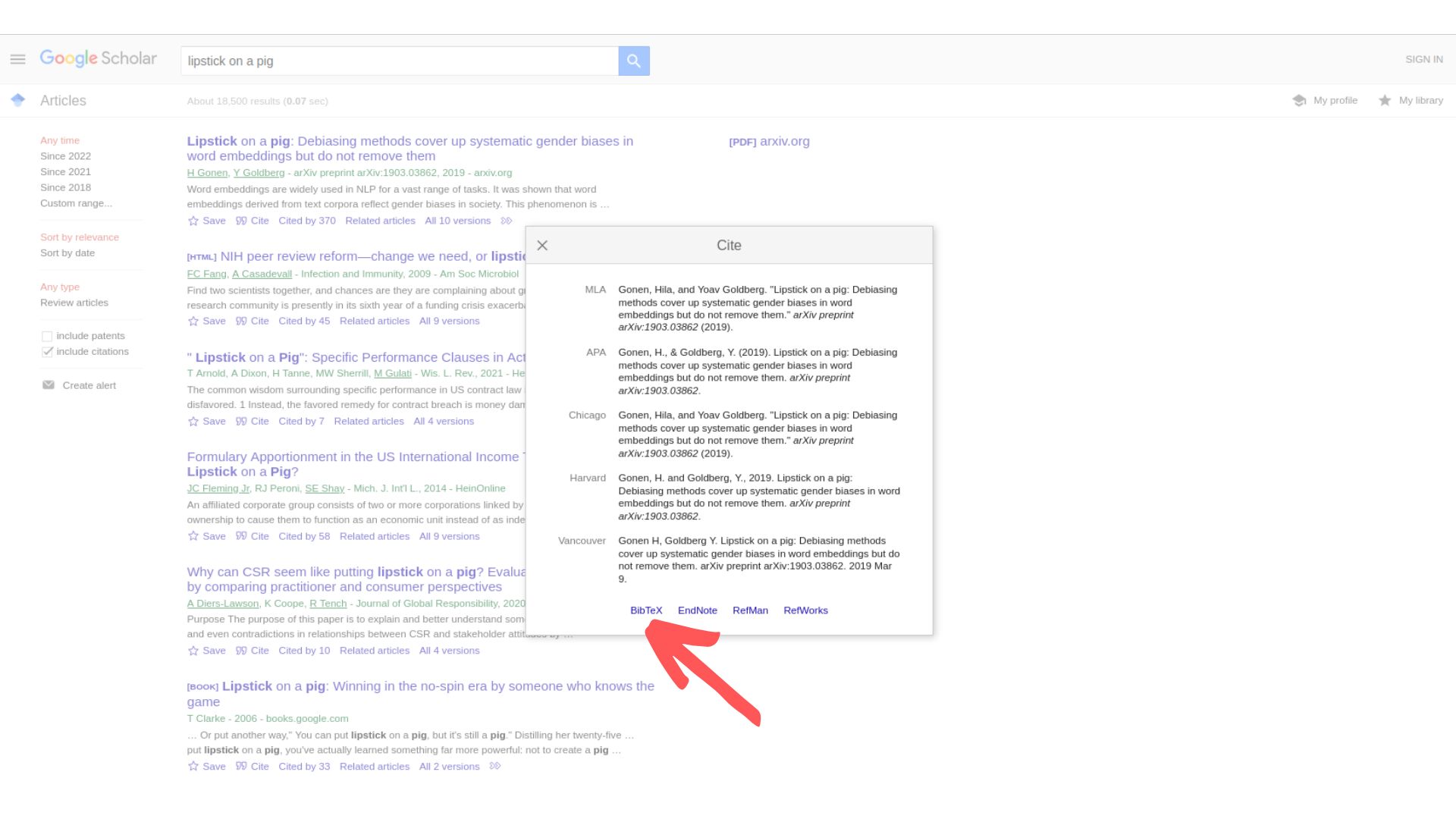

Clicking on the BibTeX link takes us to the bibliographic entry for the article. We can then copy and paste this into our .bib file (in our example, this was sample.bib).
Commenting out text
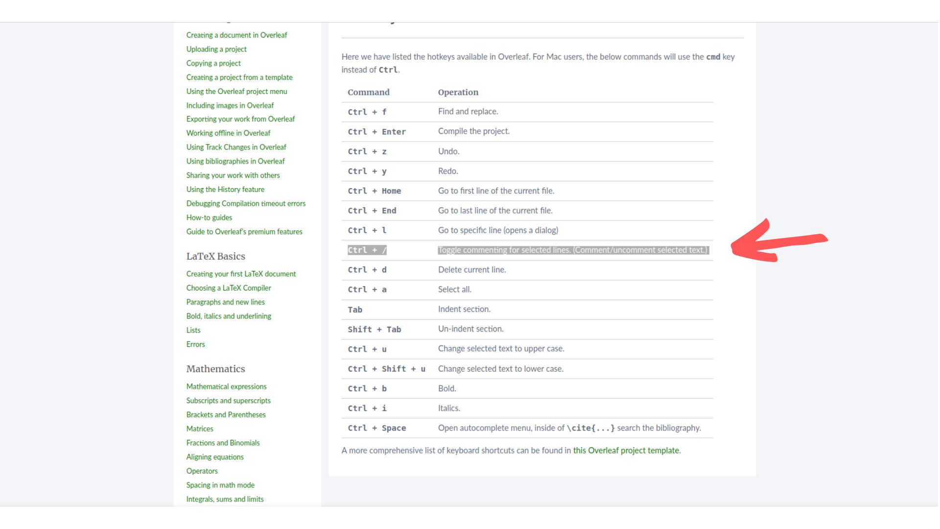
Sometimes, it’s very convenient to comment out (or in) large chunks of text in the document. It can be a little tedious to do this line by line so fortunately, there’s a shortcut for doing this in Overleaf!
Below is a screenshot from the overview of hotkeys in Overleaf! From here, we can see that if we want to toggle commenting on several lines of text at once, we can highlight the text we have in mind and then press Ctrl + / to comment or uncomment the highlighted section.
Great job!

Great job! We just went through the basics of using LaTeX to typeset documents in Overleaf! This is very useful when you want to write and make reports, notes, or presentations that involve a lot of math. For more resources on using LaTeX in Overleaf, this tutorial from Overleaf is a great place to start and also contains links to other guides on Overleaf!


